import sys
import tskit
import msprime
import pandas as pd
import numpy as np

import workshop
workbook = workshop.Simulation()
display(workbook.setup)| ✅ Your notebook is ready to go! |
To access material for this workbook please execute the notebook cell immediately below (e.g. use the shortcut +). The cell should print out “Your notebook is ready to go!”
import sys
import tskit
import msprime
import pandas as pd
import numpy as np
import workshop
workbook = workshop.Simulation()
display(workbook.setup)| ✅ Your notebook is ready to go! |
This workbook is intended to be used by executing each cell as you go along. Code cells (like those above) can be modified and re-executed to perform different behaviour or additional analysis. You can use this to complete various programming exercises, some of which have associated questions to test your understanding. Exercises are marked like this:
In this exercise we will acquaint ourselves with the extremely efficient and versatile coalescent simulator msprime. It ows much of its efficiency to the tskit (tree sequence kit) format to efficiently store and process genetic and phylogenetic data. Together with other software that use this file format, it makes up an ecosystem of high performant population genetic tools.
We will start by reproducing simulations similar to those in the previous exercise, after which we move on to more advanced examples. Many of the examples here are taken from the msprime quickstart and documentation. The idea is to familiarise yourself with the basic commands and inform you on how to find more information about functions and attributes.
Before starting the simulations, a brief review of the tskit data model is in place. The tskit storage format basically consists of a set of tables that describe the relationships between samples (nodes and edges), together with tables that describe variation (mutations and sites). The figure below (Baumdicker et al, Figure 2)) shows a concise summary of the stored information.

Here, a node corresponds to a current (time=0.0) or ancestral (time > 0.0) genome (sequence), and is stored with a unique ID in the Nodes table. An edge describes the relationship between two nodes (parent and child) and corresponds to our branches from the previous exercise. For instance, the first edge connects the node 0 (child) with its parent, node 4. Edges are stored in the Edges table and can be referenced by the nodes that they connect.
A site is a genomic position with a known ancestral state that is referenced by a unique ID and stored in the Sites table. Note that usually non-variant genomic positions (e.g., genomic positions 1 and 3) are not tracked in order to save space. A mutation is referenced by a unique ID, has a derived state, is placed on a site (corresponding to a genomic position) on a given edge (referenced by the node id) and stored in the Mutations table. Note that, somewhat confusingly perhaps, in the figure above, not all sites have associated mutations. All IDs are integers starting from 0.
Together, the site and mutation tables describe the genetic variation among the samples. The genotype matrix and the tree topologies have been derived from the tables.
Finally, in the example above, the sample variation is described by two different trees, one for (genome) position 0-10, another for position 10-20. This is a consequence of recombination having induced different genealogical histories to the left and right of the recombination breakpoint at position 10. In essence, the effect of recombination is to break sequences up into mosaics of non-recombining units, each with different (but closely related) genealogical histories, or trees. The genealogical history of a recombining chromosome can therefore be described as a sequence of trees, or tree sequence. Hence the name of tskit: tree sequence kit, a toolkit to process tree sequences.
Consult the figure when you start working with the msprime output in the exercises that follow to help you understand the concepts as we introduce them.
Briefly, coalescent simulations in msprime are done by calling two functions in succession which are called sim_ancestry and sim_mutations. In other words, we first generate genealogies, upon which we then “throw” a number of mutations, where the probability that a mutation ends up on a given branch is proportional to the relative length of that branch with respect to the total tree branch length.
Let’s first simulate the ancestry of 5 samples. The call to msprime.sim_ancestry will return a so-called tree sequence, which we will call ts.
ts = msprime.sim_ancestry(samples=5, ploidy=1, random_seed=123456)By default, msprime assumes a ploidy of 2, which is why we have to manually pass the ploidy parameter to emulate haploid simulations. In addition, by setting the random_seed, we make sure simulation output can be reproduced. Let’s print the output object:
ts| Trees | 1 |
| Sequence Length | 1 |
| Time Units | generations |
| Sample Nodes | 5 |
| Total Size | 2.0 KiB |
| Metadata | No Metadata |
| Table | Rows | Size | Has Metadata |
|---|---|---|---|
| Edges | 8 | 264 Bytes | |
| Individuals | 5 | 164 Bytes | |
| Migrations | 0 | 8 Bytes | |
| Mutations | 0 | 16 Bytes | |
| Nodes | 9 | 260 Bytes | |
| Populations | 1 | 224 Bytes | ✅ |
| Provenances | 1 | 1008 Bytes | |
| Sites | 0 | 16 Bytes |
| Provenance Timestamp | Software Name | Version | Command | Full record |
|---|---|---|---|---|
| 18 September, 2025 at 10:18:25 PM | msprime | 1.3.4 | sim_ancestry | Detailsdictschema_version: 1.0.0
software:
dictname: msprimeversion: 1.3.4
parameters:
dictcommand: sim_ancestrysamples: 5 demography: None sequence_length: None discrete_genome: None recombination_rate: None gene_conversion_rate: None gene_conversion_tract_length: None population_size: None ploidy: 1 model: None initial_state: None start_time: None end_time: None record_migrations: None record_full_arg: None additional_nodes: None coalescing_segments_only: None num_labels: None random_seed: 123456 replicate_index: 0
environment:
dict
os:
dictsystem: Linuxnode: runnervmf4ws1 release: 6.11.0-1018-azure version: #18~24.04.1-Ubuntu SMP Sat Jun 28 04:46:03 UTC 2025 machine: x86_64
python:
dictimplementation: CPythonversion: 3.11.9
libraries:
dict
kastore:
dictversion: 2.1.1
tskit:
dictversion: 0.6.4
gsl:
dictversion: 2.7 |
The ts object is an instance of the Tree Sequence class (you can also click on the link in the representation to access the help pages). If this sounds unfamiliar, think of a class as a definition (“recipe”) of a data structure that holds data, together with attributes that access the data and functions that process the data. A class is an abstract definition, so to make use of it we need to be populate it with data (instantiation). An object is therefore an actual concrete realization (instance) of a given class, like the ts object above. Looking closer at ts will hopefully make things clearer.
Briefly, ts consists of metadata, such as the Sequence Length or Time Units, and a number of tables, such as the Edges (equivalent to tree branches), Nodes, and Mutations. The metadata and table entries can be accessed with identically-named properties or functions on ts (in lowercase and where spaces have been replaced by underscores), e.g.,
print(ts.sequence_length)
print(ts.time_units)
for ind in ts.individuals():
    print(ind)
1.0
generations
Individual(id=0, flags=0, location=array([], dtype=float64), parents=array([], dtype=int32), nodes=array([0], dtype=int32), metadata=b'')
Individual(id=1, flags=0, location=array([], dtype=float64), parents=array([], dtype=int32), nodes=array([1], dtype=int32), metadata=b'')
Individual(id=2, flags=0, location=array([], dtype=float64), parents=array([], dtype=int32), nodes=array([2], dtype=int32), metadata=b'')
Individual(id=3, flags=0, location=array([], dtype=float64), parents=array([], dtype=int32), nodes=array([3], dtype=int32), metadata=b'')
Individual(id=4, flags=0, location=array([], dtype=float64), parents=array([], dtype=int32), nodes=array([4], dtype=int32), metadata=b'')So, an individual carries an id, a unique number that identifies the individual. This is a common feature of the tskit data structures in that all objects carry a unique numeric identifier id that starts from 0. Furthermore, there are references to an individual’s parents, which is a list of integers corresponding to parent ids, and similarly for nodes, the nodes of the tree. Finally, there is additional information such as a metadata slot.
The ts.individuals() function accesses individuals from the Individuals table, one by one. As we here have simulated a small genealogy, you can also print the table directly (but don’t do it for large simulations!):
ts.tables.individuals| id | flags | location | parents | metadata |
|---|---|---|---|---|
| 0 | 0 | |||
| 1 | 0 | |||
| 2 | 0 | |||
| 3 | 0 | |||
| 4 | 0 |
In addition to the properties and functions that map to the metadata and table names, there are a number of convenience functions that provide shortcut access to quantities of interest, e.g., ts.num_individuals and ts.num_populations:
ts.num_individuals, ts.num_populations(5, 1)You can find all properties and functions defined on ts by using the Python builtin dir:
dir(ts)There (of course) exists functionality to easily plot a genealogy. The ts object has several draw_ functions, on of which produces svg output:
ts.draw_svg()
Apart from showing the genealogy, there is a genome coordinate system, showing the simulations assume a sequence of length 1 nucleotide by default.
Now that we have a genealogy, we add mutations with a sim_mutations function, msprime.sim_mutations:
mutated_ts = msprime.sim_mutations(ts, rate=0.5, random_seed=54321)Here, we specify the mutation rate via the rate parameter, which according to the docs is “The rate of mutation per unit of sequence length per unit time” (try varying this parameter and see how it affects the illustrated genealogy below):
mutated_ts.draw_svg(size=(500, 300))
Here we increase the size of the plot to see the details better. To begin with, a mutation is indicated with a red x. In addition, the mutations are numbered, such that the ordering along a genetic sequence is explicit. Finally, at genome position 0 you see ∨ marks that indicate the position of a mutation.
The latter point can also be illustrated by printing all the mutations, as follows (note the information in site):
for mut in mutated_ts.mutations():
    print(mut)
Mutation(id=0, site=0, node=3, derived_state='T', parent=-1, metadata=b'', time=3.185986172229537, edge=6)
Mutation(id=1, site=0, node=6, derived_state='G', parent=-1, metadata=b'', time=0.9840215241955003, edge=5)
Mutation(id=2, site=0, node=3, derived_state='G', parent=0, metadata=b'', time=0.8323690266716649, edge=6)
Mutation(id=3, site=0, node=5, derived_state='T', parent=-1, metadata=b'', time=0.6321303182614809, edge=4)
Mutation(id=4, site=0, node=5, derived_state='C', parent=3, metadata=b'', time=0.4845532035498001, edge=4)As before, there are shorthand functions and properties to access quantities of interest, e.g.,
workbook.question("mutation_site")mutated_ts.tables.sites| id | position | ancestral_state | metadata |
|---|---|---|---|
| 0 | 0 | C |
There is support for calculating a variety of summary statistics on tree sequences. For instance, to calculate the diversity of mutated_ts you can run
mutated_ts.diversity()0.6So far we have basically demonstrated how our homemade simulations look in msprime. However, the msprime versions of sim_ancestry and sim_mutations provide many more options than our functions, and simulations can accomodate much more complex and realistic scenarios, such as recombination, migration, demographic changes, in some cases selection, and more. Briefly skim the API documentation by following the links above to get an overview of what these functions can do.
Until now, we have focused on haploid individuals. In order to introduce recombination, we shift to diploids, which is in fact the default setting in msprime. Begin by simulating a small tree consisting of two samples.
ts = msprime.sim_ancestry(samples=2, random_seed=23423)
ts.draw_svg(size=(500, 300))
As the tree shows, we have four terminal nodes (leaves) with ids 0-3, but we only specified two samples. Why? Recall that a node corresponds to a chromosome. Since we are simulating diploid individuals, there are two chromosome per individual, i.e., two nodes per individual. The sim_ancestry documentation states that samples indeed correspond to individuals, and consequently the number of terminal nodes will be the sample size times the ploidy.
The relationship between nodes and individuals can at first be confusing. The tskit documentation section Nodes, genomes or individuals? briefly discusses the distinction between these entities.
workbook.question("individual_node")By default sequences in msprime correspond to nucleotides. Let’s specify a 10kb sequence with the parameter sequence_length. Note how the genome coordinates change in the resulting plot. Note also that by using the same random seed as above, the genealogy remains unchanged.
ts = msprime.sim_ancestry(samples=2,
                          sequence_length=10_000,
                          random_seed=23423)
ts.draw_svg(size=(500, 300))
Sofar the tree sequence consists of one tree, which corresponds to a non-recombining sequence. We can set the recombination_rate parameter to add recombination. Note how we now have three trees, one for each non-recombining sequence.
ts = msprime.sim_ancestry(samples=2,
                          sequence_length=10_000,
                          recombination_rate=1e-5, # set a high rate
                          random_seed=12353
                         )
ts.draw_svg(size=(600, 300))
workbook.question("recombination")Sofar, we have not mentioned population size in our simulations, but this is something we would like to do since this parameter affects the dynamics of the system. We can set the population size with the population_size option, which corresponds to the effective population size \(N_e\). Note that we decrease the sequence length and recombination rate to speed up simulation:
ts_small = msprime.sim_ancestry(
    samples=2,
    sequence_length=1_000,
    recombination_rate=1e-8,
    population_size=20_000, # similar to human Ne
    random_seed=12123
)
ts_small.draw_svg()
To demonstrate the speed of msprime, simulate a large tree sequence of 20,000 diploid individuals with 1Mbp genomes and a recombination rate of 1e-8. Use the random seed 42, save the output to a variable large_ts and print the table.
# Exercise 2: Set `large_ts` to a new large tree sequence, generated
# using msprime.sim_ancestry() with specific parameters
# (random_seed=42, etc.), then output the tree sequence summary table
# to screen.workbook.question("large_ancestry")Now we add mutations to the simulated ancestry. Note that there are more mutations than sites.
mts_small = msprime.sim_mutations(
    ts_small, # Use the small tree so we can visualize mutations
    rate=1e-7, # set a high mutation rate
    random_seed=22
)mts_small.draw_svg(size=(600, 300))
Print out the mutations table of the mts_small object.
workbook.question("mutation_id")We’ll now add mutations to the large ancestry simulated previously. Recall that we have a sample size of 20,000, corresponding to 40,000 chromosomes. A 1Mbp sequence may contain in the order of 10,000 variant positions, which in a Variant Call Format (vcf) file would constitute a 40,000 by 10,000 matrix, requiring ca 700 Mb (uncompressed) storage. The resulting tree sequence, however, only requires 8Mb.
<dd>large_ts tree sequence simulated previously. Use a random seed 276 and mutation rate 1e-8.
# Exercise 4: add mutations to large_ts with random seed 276 and
# mutation rate 1e-8
%time # Time the command
CPU times: user 2 μs, sys: 0 ns, total: 2 μs
Wall time: 5.25 μsworkbook.question("large_mutation")Note that it only takes a second or two two generate this reasonably large data set which fits handily on a laptop. With the efficient storage that the tskit library provide, together with efficient simulators like msprime, it is now possible to simulate data for realistically large populations and genome sizes
We end by demonstrating one of the practical uses of simulation (apart from the pedagogical utility). We will in upcoming exercises work on monkeyflowers to describe observed patterns of variation and diversity. The goal is to build a model that explains how the observed variation has been shaped by a combination of demographic history, selection, migration, and other processes. Whatever the methodology may be, the unifying principle is that trees are estimated together with a mutation process that explains the variation. This is true even if tree estimation is not always explicitly mentioned, since all summary statistics can be rephrased in the context of trees.
In the study Widespread selection and gene flow shape the genomic landscape during a radiation of monkeyflowers, the authors use SLiM to simulate a parental population of size N=10,000, that after 10N generations split into 2 daughter populations, each of size N, that continued evolving 10N generations. They simulated a 21Mbp chromosome with a recombination rate of \(1.5 \times 10^{-8}\) and a mutation rate of \(10^{-8}\), both per base pair and per generation.
We will make a slightly smaller simulation here in the case of a neutrally evolving population; coalescent simulations cannot be used to model but the simplest models of selections (e.g., sweeps). Since we will look at a 3Mbp, let’s simulate a region of this size. In order to model the demography, we need to make use of the msprime.Demography class. The parameter and function names should be self-explanatory in the example below.
N = 10_000
# Instantiate an empty msprime.Demography object
demography = msprime.Demography()
# Add populations with reasonable names
demography.add_population(name="ancestral", initial_size=N)
demography.add_population(name="red", initial_size=N)
demography.add_population(name="yellow", initial_size=N)
# Add time of population split where we define derived and ancestral populations
demography.add_population_split(time=10*N, derived=["red", "yellow"],
                                ancestral="ancestral")
PopulationSplit(time=100000, derived=['red', 'yellow'], ancestral='ancestral')We can print information about the demography with the demography.debug function:
# Print information about the demography
demography.debug()| start | end | growth_rate | red | yellow | |
|---|---|---|---|---|---|
| red | 10000.0 | 10000.0 | 0 | 0 | 0 |
| yellow | 10000.0 | 10000.0 | 0 | 0 | 0 |
| time | type | parameters | effect |
|---|---|---|---|
| 1e+05 | Population Split | derived=[red, yellow], ancestral=ancestral | Moves all lineages from derived populations 'red' and 'yellow' to the ancestral 'ancestral' population. Also set the derived populations to inactive, and all migration rates to and from the derived populations to zero. |
| start | end | growth_rate | |
|---|---|---|---|
| ancestral | 10000.0 | 10000.0 | 0 |
Briefly, the printed information shows we have two epochs, that are printed in reverse chronological order (most recent epoch first). The first epoch (index 0) goes from current time (0) to 1e+05 generations ago, the second from 1e+05 generations ago back in time towards infinity (when all lineages have coalesced). At generation 1e+05 (time ago) there was a population split from the ancestral population to the red and yellow populations.
An alternative, and perhaps more instructive way to summarize the demography, is to use the nifty demesdraw to plot it:
import demesdraw
import matplotlib.pyplot as plt

graph = msprime.Demography.to_demes(demography)
fig, ax = plt.subplots()
demesdraw.tubes(graph, ax=ax, seed=1)
plt.show()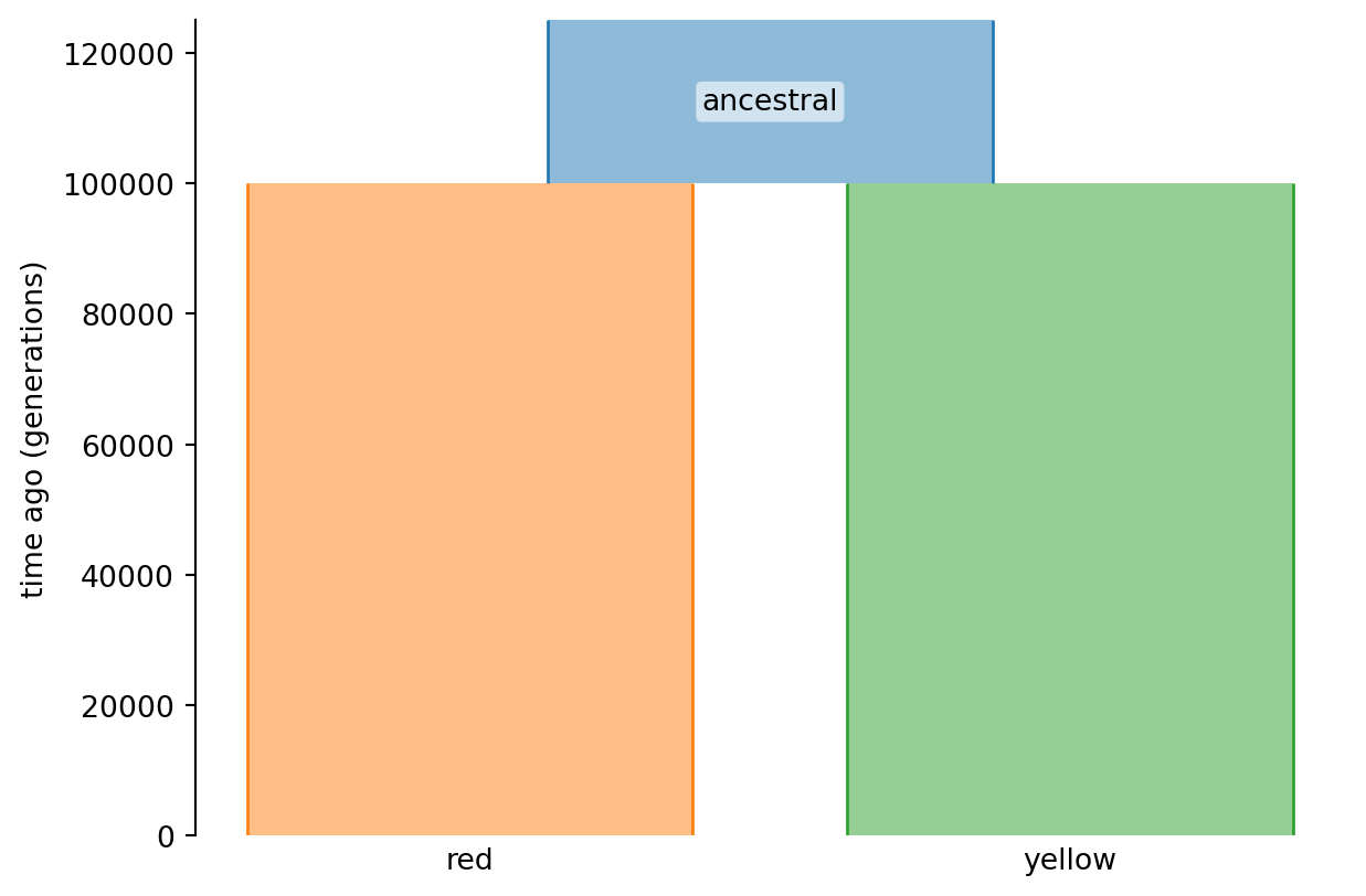
Now that we have defined the demographic model, we can simulate the ancestry on top of this model by passing the demography option. In addition, we specify the number of samples by population by passing a Python dictionary; briefly, this is a “key”:value mapping enclosed in curly brackets.
ts = msprime.sim_ancestry(
    samples={"red": 5, "yellow": 5},
    demography=demography, random_seed=12,
    sequence_length=3_000_000,
    recombination_rate=1.5e-8,
)
ts| Trees | 10 213 |
| Sequence Length | 3 000 000 |
| Time Units | generations |
| Sample Nodes | 20 |
| Total Size | 1.4 MiB |
| Metadata | No Metadata |
| Table | Rows | Size | Has Metadata |
|---|---|---|---|
| Edges | 32 947 | 1.0 MiB | |
| Individuals | 10 | 304 Bytes | |
| Migrations | 0 | 8 Bytes | |
| Mutations | 0 | 16 Bytes | |
| Nodes | 6 746 | 184.5 KiB | |
| Populations | 3 | 309 Bytes | ✅ |
| Provenances | 1 | 1.7 KiB | |
| Sites | 0 | 16 Bytes |
| Provenance Timestamp | Software Name | Version | Command | Full record |
|---|---|---|---|---|
| 18 September, 2025 at 10:18:26 PM | msprime | 1.3.4 | sim_ancestry | Detailsdictschema_version: 1.0.0
software:
dictname: msprimeversion: 1.3.4
parameters:
dictcommand: sim_ancestry
samples:
dictred: 5yellow: 5
demography:
dict
populations:
listdictinitial_size: 10000growth_rate: 0 name: ancestral description:
extra_metadata:
dictdefault_sampling_time: 100000 initially_active: False id: 0 dictinitial_size: 10000growth_rate: 0 name: red description:
extra_metadata:
dictdefault_sampling_time: None initially_active: None id: 1 dictinitial_size: 10000growth_rate: 0 name: yellow description:
extra_metadata:
dictdefault_sampling_time: None initially_active: None id: 2
events:
listdicttime: 100000
derived:
listredyellow ancestral: ancestral
migration_matrix:
listlist0.00.0 0.0 list0.00.0 0.0 list0.00.0 0.0 __class__: msprime.demography.Demography sequence_length: 3000000 discrete_genome: None recombination_rate: 1.5e-08 gene_conversion_rate: None gene_conversion_tract_length: None population_size: None ploidy: None model: None initial_state: None start_time: None end_time: None record_migrations: None record_full_arg: None additional_nodes: None coalescing_segments_only: None num_labels: None random_seed: 12 replicate_index: 0
environment:
dict
os:
dictsystem: Linuxnode: runnervmf4ws1 release: 6.11.0-1018-azure version: #18~24.04.1-Ubuntu SMP Sat Jun 28 04:46:03 UTC 2025 machine: x86_64
python:
dictimplementation: CPythonversion: 3.11.9
libraries:
dict
kastore:
dictversion: 2.1.1
tskit:
dictversion: 0.6.4
gsl:
dictversion: 2.7 |
Finally, we add mutations as before:
mut_ts = msprime.sim_mutations(ts, rate=1e-8, random_seed=12)Before we start calculating summary statistics, we need to define so-called sample sets which group samples in populations. Intuitively, on may want to assign individual ids to sample sets, but if you look at the populations and individuals tables, you will note that there is no direct link between individuals and populations. The mapping we really need is from nodes to populations. We look directly at the nodes table, recalling that ancestral nodes map to individuals with id -1:
# Subset the nodes table (6746 rows!) to leaf nodes
ts.tables.nodes[ts.tables.nodes.individual > -1]| id | flags | population | individual | time | metadata |
|---|---|---|---|---|---|
| 0 | 1 | 1 | 0 | 0 | |
| 1 | 1 | 1 | 0 | 0 | |
| 2 | 1 | 1 | 1 | 0 | |
| 3 | 1 | 1 | 1 | 0 | |
| 4 | 1 | 1 | 2 | 0 | |
| 5 | 1 | 1 | 2 | 0 | |
| 6 | 1 | 1 | 3 | 0 | |
| 7 | 1 | 1 | 3 | 0 | |
| 8 | 1 | 1 | 4 | 0 | |
| 9 | 1 | 1 | 4 | 0 | |
| 10 | 1 | 2 | 5 | 0 | |
| 11 | 1 | 2 | 5 | 0 | |
| 12 | 1 | 2 | 6 | 0 | |
| 13 | 1 | 2 | 6 | 0 | |
| 14 | 1 | 2 | 7 | 0 | |
| 15 | 1 | 2 | 7 | 0 | |
| 16 | 1 | 2 | 8 | 0 | |
| 17 | 1 | 2 | 8 | 0 | |
| 18 | 1 | 2 | 9 | 0 | |
| 19 | 1 | 2 | 9 | 0 |
As one would expect, node ids 0-9 map to population id=1 (red), whereas node ids 10-19 map to population id=2 (yellow). We use this information to define the sample sets (basically, we assign individual ids to different groupings). Although we could do it by listing all the node ids, there is a more convenient way of defining the sample sets:
sample_sets = [mut_ts.samples(population=1), mut_ts.samples(population=2)]
sample_sets
[array([0, 1, 2, 3, 4, 5, 6, 7, 8, 9], dtype=int32),
array([10, 11, 12, 13, 14, 15, 16, 17, 18, 19], dtype=int32)]The sample_sets variable is a list of lists, where each sublist is a list of node ids. Note that although this particular grouping is based on population labels, we could partition the nodes in any way we want, e.g., by geographic coordinates if they are available, or other information that hints at other ways of grouping samples.
We end by calculating and plotting some summary statistics for the data, both for all samples, and grouped by population, which is easily done by passing the sample_sets option. Below we show examples for diversity (\(\pi\)), divergence (\(d_{XY}\)), and \(F_{ST}\). For a complete list of statistics, see https://tskit.dev/tskit/docs/stable/stats.html#statistics.
msprime_results = {}
msprime_results["pi"] = mut_ts.diversity()
msprime_results["pi0"] = mut_ts.diversity(sample_sets=sample_sets[0])
msprime_results["pi1"] = mut_ts.diversity(sample_sets=sample_sets[1])
msprime_results["div"] = mut_ts.divergence(sample_sets=sample_sets)
msprime_results["fst"] = mut_ts.Fst(sample_sets=sample_sets)
msprime_results
{'pi': 0.0014349508771930018,
'pi0': 0.0003837407407407586,
'pi1': 0.00041549629629631773,
'div': 0.0023667500000000463,
'fst': 0.711088008814865}We can also calculated windowed statistics and plot them along the simulated chromosome. Here, we show an example for Fst, where we define 100 windows, equivalent to a window size of 30kbp.
num_windows=100
window_size = mut_ts.sequence_length / num_windows
# Generate window coordinates from 0 to sequence length
windows=np.linspace(0, mut_ts.sequence_length, num_windows + 1)
fst = mut_ts.Fst(sample_sets=sample_sets, windows=windows)
# Translate window index to genome position
x = [window_size*x for x in range(len(windows) - 1)]
plt.plot(x, fst)
plt.xlabel("Genome position (bp)")
plt.ylabel("Fst")
plt.show()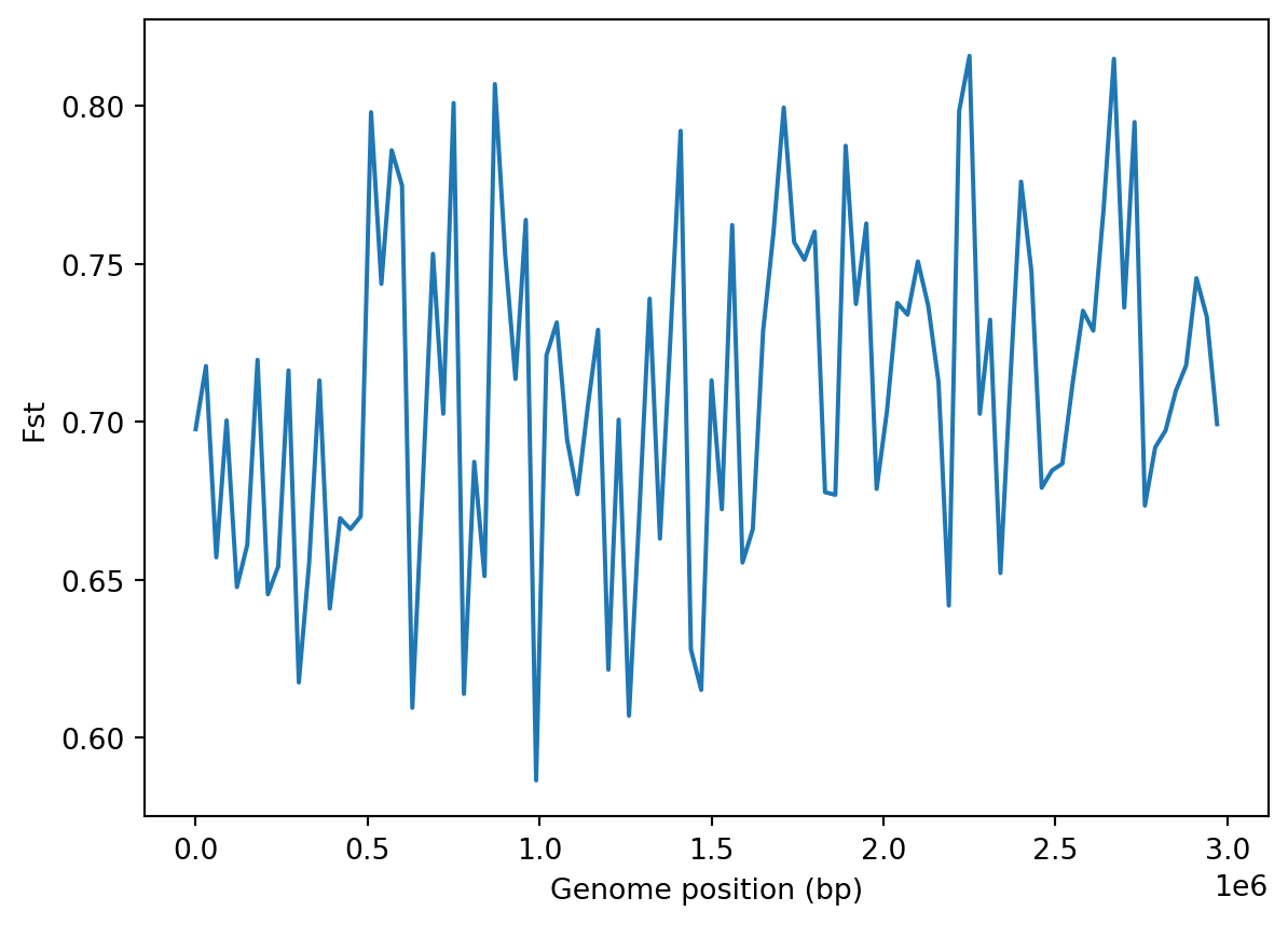
Do these numbers make sense? Let’s compare the results with the simulations performed by the authors who, as you may recall, used SLiM for their simulations. You can download the windowed statistics from the original publication like so:
url = "https://raw.githubusercontent.com/mufernando/mimulus_sims/master/data/raw_stats.csv"
if "pyodide" in sys.modules:
from pyodide.http import open_url
raw_stats = open_url(url)
data = pd.read_csv(raw_stats)
else:
data = pd.read_csv(url)Each row corresponds to a simulation time point for a given parameter setting. We first subset the data to look only at the results from the neutral simulation:
df = data[data.label.str.startswith("Neutral")]
df| Unnamed: 0 | N | non_neutral_mu | rec | L | L0 | L1 | m | ndeff | nprop | ... | fst_win_33 | fst_win_34 | fst_win_35 | fst_win_36 | fst_win_37 | fst_win_38 | fst_win_39 | fst_win_40 | fst_win_41 | fst_win_42 | |
|---|---|---|---|---|---|---|---|---|---|---|---|---|---|---|---|---|---|---|---|---|---|
| 240 | 190 | 10000.0 | 0.0 | 2.000000e-08 | 21000000.0 | 7000000.0 | 7000000.0 | 0.0 | 0.0 | 0.0 | ... | 0.000133 | 0.000045 | 0.000072 | 0.000088 | 0.000066 | 0.000050 | 0.000079 | 0.000106 | 0.000092 | 0.000126 |
| 241 | 191 | 10000.0 | 0.0 | 2.000000e-08 | 21000000.0 | 7000000.0 | 7000000.0 | 0.0 | 0.0 | 0.0 | ... | 0.165958 | 0.184471 | 0.157133 | 0.154071 | 0.158101 | 0.136834 | 0.149252 | 0.149664 | 0.197518 | 0.153251 |
| 242 | 192 | 10000.0 | 0.0 | 2.000000e-08 | 21000000.0 | 7000000.0 | 7000000.0 | 0.0 | 0.0 | 0.0 | ... | 0.246486 | 0.284898 | 0.269796 | 0.235144 | 0.290248 | 0.277218 | 0.284167 | 0.284734 | 0.314286 | 0.319089 |
| 243 | 193 | 10000.0 | 0.0 | 2.000000e-08 | 21000000.0 | 7000000.0 | 7000000.0 | 0.0 | 0.0 | 0.0 | ... | 0.367805 | 0.373784 | 0.354475 | 0.334356 | 0.360815 | 0.318182 | 0.391959 | 0.402007 | 0.348054 | 0.381364 |
| 244 | 194 | 10000.0 | 0.0 | 2.000000e-08 | 21000000.0 | 7000000.0 | 7000000.0 | 0.0 | 0.0 | 0.0 | ... | 0.454584 | 0.462483 | 0.414050 | 0.433806 | 0.423987 | 0.391511 | 0.506720 | 0.466908 | 0.427348 | 0.476698 |
| 245 | 195 | 10000.0 | 0.0 | 2.000000e-08 | 21000000.0 | 7000000.0 | 7000000.0 | 0.0 | 0.0 | 0.0 | ... | 0.502353 | 0.471698 | 0.490566 | 0.477353 | 0.502021 | 0.454525 | 0.550316 | 0.519354 | 0.514579 | 0.522261 |
| 246 | 196 | 10000.0 | 0.0 | 2.000000e-08 | 21000000.0 | 7000000.0 | 7000000.0 | 0.0 | 0.0 | 0.0 | ... | 0.647825 | 0.684596 | 0.644272 | 0.672648 | 0.693862 | 0.668499 | 0.683258 | 0.685237 | 0.666588 | 0.666856 |
| 247 | 197 | 10000.0 | 0.0 | 2.000000e-08 | 21000000.0 | 7000000.0 | 7000000.0 | 0.0 | 0.0 | 0.0 | ... | 0.744313 | 0.754212 | 0.755121 | 0.743564 | 0.756233 | 0.741642 | 0.735638 | 0.747693 | 0.760965 | 0.741939 |
| 248 | 198 | 10000.0 | 0.0 | 2.000000e-08 | 21000000.0 | 7000000.0 | 7000000.0 | 0.0 | 0.0 | 0.0 | ... | 0.795313 | 0.787214 | 0.803706 | 0.800828 | 0.781259 | 0.805021 | 0.791966 | 0.804775 | 0.775935 | 0.795137 |
| 249 | 199 | 10000.0 | 0.0 | 2.000000e-08 | 21000000.0 | 7000000.0 | 7000000.0 | 0.0 | 0.0 | 0.0 | ... | 0.835605 | 0.827921 | 0.821808 | 0.819095 | 0.815445 | 0.832035 | 0.830157 | 0.837417 | 0.818819 | 0.822238 |
10 rows × 182 columns
Window statistics are in columns labelled statistic_win_number, where the statistics are diversity \(\pi\) (“pi0” for population 0, “pi1” for population 1), divergence (“div”), and fst (“fst”). The “T” column corresponds to time points indices; the actual times are expressed in terms of population size N as follows (one has to look at the jupyter notebook analysis.ipynb in the source code directory that accompanies the publication to see this):
T=np.concatenate([np.arange(0,2.2,step=0.4), np.arange(4,11,step=2)])
T = [float("%.1f"%t) for t in T]
T[0.0, 0.4, 0.8, 1.2, 1.6, 2.0, 4.0, 6.0, 8.0, 10.0]We will only concern ourselves with the last timepoint here (index 9), which corresponds to the current time in terms of the simulation:
results = {}
for stat in ["pi0", "pi1", "div", "fst"]:
x = np.mean(df[df["T"] == 9][df.columns[df.columns.str.startswith(stat)]])
results[stat] = x
results, msprime_results({'pi0': 0.0003987941886562929,
'pi1': 0.00040107865412194283,
'div': 0.002373768495238081,
'fst': 0.8313226980660732},
{'pi': 0.0014349508771930018,
 'pi0': 0.0003837407407407586,
 'pi1': 0.00041549629629631773,
 'div': 0.0023667500000000463,
'fst': 0.711088008814865})We see that the results are mostly similar to those that we obtained, which is reassuring, as msprime and SLiM should not differ under the neutral model. However, the exception is \(F_{ST}\). This has to do with how msprime and SLiM calculate \(F_{ST}\). msprime uses the expression \(F_{ST} = 1 - 2(\pi_0 + \pi_1)/(\pi_0 + 2d_{XY} + \pi_1)\), whereas SLiM (seems to) uses the expression \(F_{ST} = 1 - \frac{(\pi_0 + \pi_1)/2}{d_{XY}}\). Let’s check these expressions below.
For msprime we have:
1 - 2 * (msprime_results["pi0"] + msprime_results["pi1"]) / \
    (msprime_results["pi0"] + msprime_results["pi1"] + \
2*msprime_results["div"])0.711088008814865For SLiM:
1 - ((results["pi0"] + results["pi1"]) / 2) / results["div"]0.8315183548052754Comparing these results with those above shows that the discrepancy in \(F_{ST}\) can be explained by differences in how it is calculated. This echoes what Alistair Miles, the author of scikit-allel, has to say about \(F_{ST}\):
FST is a statistic which seems simple at first yet quickly becomes very technical when you start reading the literature
Amen.