
Primer on the coalescent and forward simulation
The Wright-Fisher model and simulations
Recap
Model of a population describing genealogies under the following assumptions
- discrete and non-overlapping generations
- haploid individuals or two subpopulations (males and females)
- constant population size
- all individuals are equally fit
- population has no geographical or social structure
- no recombination
Forward simulation
The Wright-Fisher model and simulations


Mean reproductive success = 63.4%. Can show for large populations P(no descendants)=1 - e^{-1} \approx 0.632
Forward and backward simulation


Simulated nodes are filled with black. Genealogy of interest is highlighted in thick black lines.
Coalescent simulations
The coalescent simulates the genealogy of a sample of individuals on which mutations are “sprinkled” according to a Poisson process.
- Simulate ancestry (genealogy)

Coalescent simulations
The coalescent simulates the genealogy of a sample of individuals on which mutations are “sprinkled” according to a Poisson process.
- Simulate ancestry (genealogy)
- Simulate mutations

Coalescent simulations
The coalescent simulates the genealogy of a sample of individuals on which mutations are “sprinkled” according to a Poisson process.
- Simulate ancestry (genealogy)
- Simulate mutations
Exercise
How many mutations are common to all samples? How many mutations does sample 1 have? Sample 2?
Assuming the ancestral state is denoted 0 (prior to the first generation) and the derived state 1, what are the sequences of the samples?

Simulating genealogies (Hahn, 2019, p. 115)
- Start with i=n chromosomes

Simulating genealogies (Hahn, 2019, p. 115)
Start with i=n chromosomes
Choose time to next coalescent event from an exponential distribution with parameter \lambda=i(i-1)/2

Simulating genealogies (Hahn, 2019, p. 115)
Start with i=n chromosomes
Choose time to next coalescent event from an exponential distribution with parameter \lambda=i(i-1)/2
Choose two chromosomes at random to coalesce

Simulating genealogies (Hahn, 2019, p. 115)
Start with i=n chromosomes
Choose time to next coalescent event from an exponential distribution with parameter \lambda=i(i-1)/2
Choose two chromosomes at random to coalesce
Merge the two lineages and set i \rightarrow i - 1

Simulating genealogies (Hahn, 2019, p. 115)
- Start with i=n chromosomes
- Choose time to next coalescent event from an exponential distribution with parameter \lambda=i(i-1)/2
- Choose two chromosomes at random to coalesce
- Merge the two lineages and set i \rightarrow i - 1
- If i>1, go to step 2; if not, stop.

Simulating genealogies (Hahn, 2019, p. 115)
- Start with i=n chromosomes
- Choose time to next coalescent event from an exponential distribution with parameter \lambda=i(i-1)/2^1
- Choose two chromosomes at random to coalesce
- Merge the two lineages and set i \rightarrow i - 1
- If i>1, go to step 2; if not, stop.
^1: The exponential can be parametrized in two different ways, so that the parameter to the function is either \lambda or \beta=1/\lambda.

Some properties of the tree

The waiting time for coalescence is shorter when there are more lineages
Time to the most recent common ancestor (MRCA) (i.e., the tree height) is the sum of the waiting times (T_2 + T_3 + ...)
On average, the time for coalescence when there are two remaining lineages is half the tree height
Diminishing returns of adding more samples

Adding mutations

Mutations are added by “throwing” them on branches, where the probability of ending up on a given branch is equal to its relative length.
The total number of segregating sites S to be thrown on the tree is modelled as a Poisson random variable which expresses the probability of a given number of events in a given time. Here the time is the total branch length of the tree and mutations are added with intensity proportional to the population mutation rate \theta.
The coalescent and diversity
| 1 | 2 | 3 | 4 | 5 | 6 | 7 | 8 | 9 | 10 | 11 | 12 | 13 | 14 | 15 |
|---|---|---|---|---|---|---|---|---|---|---|---|---|---|---|
| T | T | A | C | A | A | T | C | C | G | A | T | C | G | T |
| T | T | A | C | G | A | T | G | C | G | C | T | C | G | T |
| T | C | A | C | A | A | T | G | C | G | A | T | G | G | A |
| T | T | A | C | G | A | T | G | C | G | C | T | C | G | T |
| * | * | * | * | * | * |
\begin{align} \pi & = \sum_{j=1}^S h_j = \sum_{j=1}^{S} \frac{n}{n-1}\left(1 - \sum_i p_i^2 \right) \\ & \stackrel{S=6,\\ n=4}{=} \sum_{j=1}^{6} \frac{4}{3}\left(1 - \sum_i p_i^2\right) \\ & = \frac{4}{3}\left(\mathbf{\color{#a7c947}{4}}\left(1-\frac{1}{16}-\frac{9}{16}\right) + \mathbf{\color{#a7c947}{2}}\left(1 - \frac{1}{4} - \frac{1}{4}\right)\right) = \frac{10}{3} \end{align}


In this notation one can show that \pi, the nucleotide diversity, is
\begin{equation*} \begin{split} \pi & = \frac{\sum_{i=1}^{n-1}i(n-i)\xi_i}{n(n-1)/2} \\ & \stackrel{n=4}{=} \frac{1*(4-1)*4 + 2*(4-2)*2}{6} \\ & = \frac{10}{3} \end{split} \end{equation*}
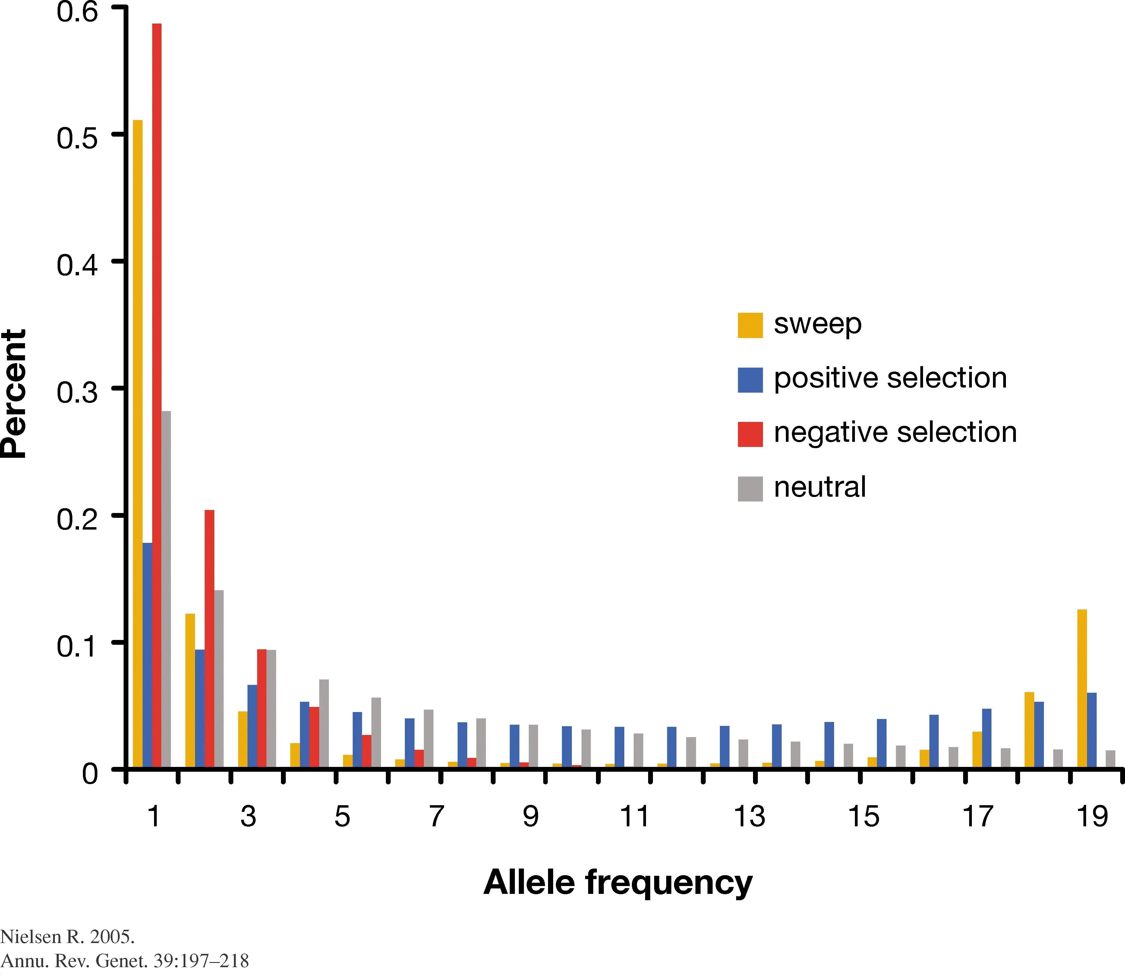
Many statistical quantities can be related to the site frequency spectrum (SFS), which is a summary of the frequencies of the segregating sites. Let \xi_i be the number of chromosomes in the sample with i minor alleles. In the example above we have S=6 mutations on n=4 chromosomes.
The impact of topology on the SFS
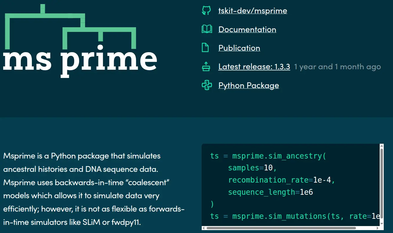
msprime

- Fast & flexible backward-time simulator
- Separates ancestry from mutation simulation
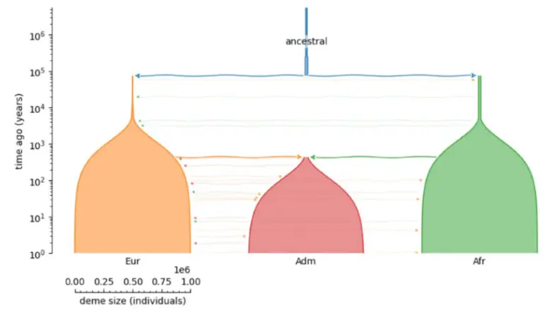
- Arbitrary discrete demographies / species
- Pedigree support (e.g., 1M+ Quebec ARG)
- Approximate extension to selective sweeps
msprime stores data as succinct tree sequences
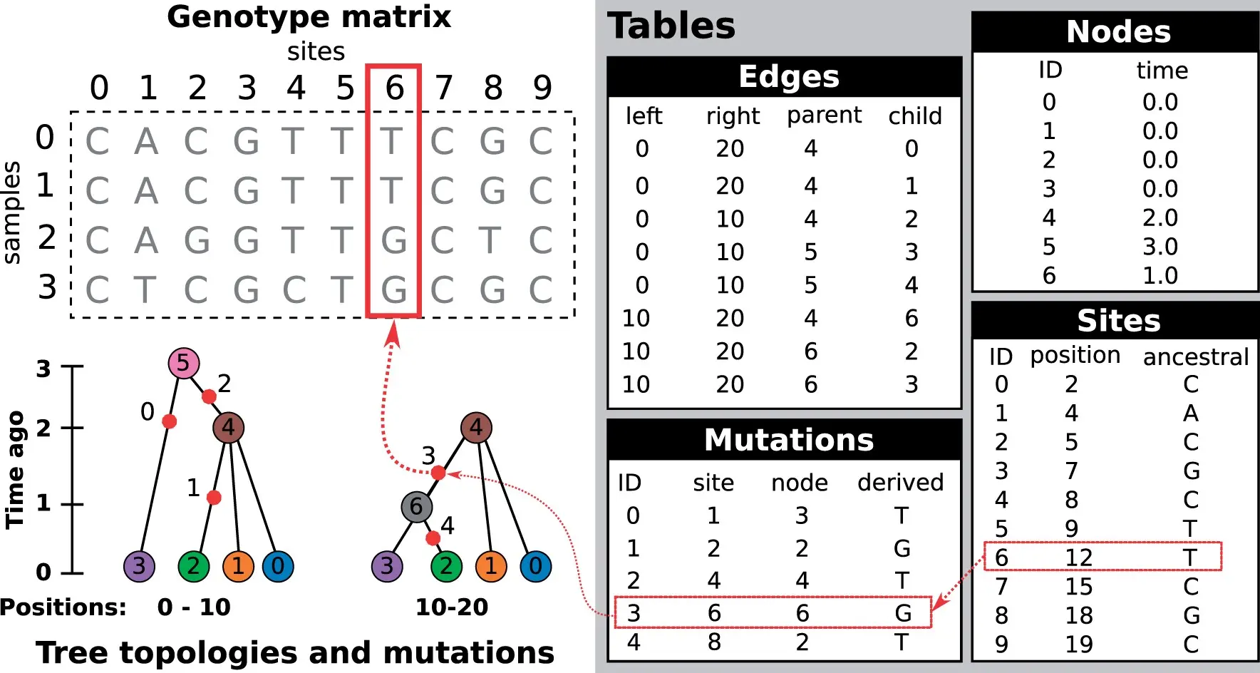
Tree sequences compress data and speedup analyses
- Compact storage (“domain specific compression”)
- Fast, efficient analysis (a “succinct” structure)
- Well tested, open source (active dev community)
Data compression

- Built-in functionality (well documented: http://tskit.dev)
…but limited support for major genomic rearrangements (e.g. inversions, large indels): genomes should be (reasonably) aligned => current primary focus = population genetics
Speed

Bibliography
Baumdicker, F., Bisschop, G., Goldstein, D., Gower, G., Ragsdale, A. P., Tsambos, G., Zhu, S., Eldon, B., Ellerman, E. C., Galloway, J. G., Gladstein, A. L., Gorjanc, G., Guo, B., Jeffery, B., Kretzschumar, W. W., Lohse, K., Matschiner, M., Nelson, D., Pope, N. S., … Kelleher, J. (2022). Efficient ancestry and mutation simulation with msprime 1.0. Genetics, 220(3), iyab229. https://doi.org/10.1093/genetics/iyab229
Hahn, M. (2019). Molecular Population Genetics (First). Oxford University Press.
Hein, J., Schierup, M. H., & Wiuf, C. (2005). Gene genealogies, variation and evolution: A primer in coalescent theory. Oxford University Press. https://books.google.se/books?id=CCmLNAEACAAJ
Wakeley, J. (2008). Coalescent Theory: An Introduction (1st Edition edition). Roberts and Company Publishers.