A generic variant calling workflow consists of the following basic steps:
read quality control and filtering
read mapping
removal / marking of duplicate reads
joint / sample-based variant calling and genotyping
There are different tweaks and additions to each of these steps, depending on application and method.
1. Read quality control
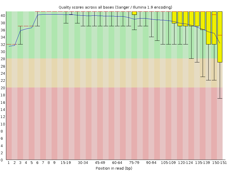
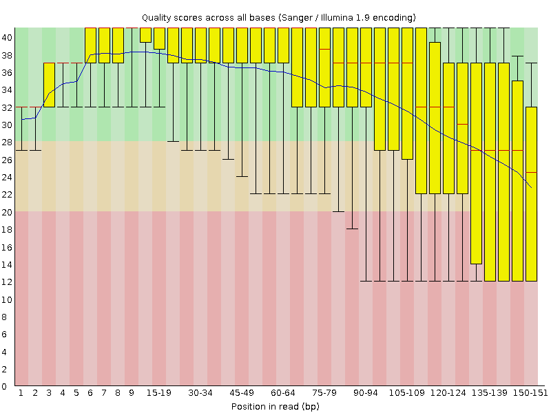
Figure 1: Per base quality scores, read 1 (upper) and read 2 (lower panel), obtained from the FastQC program. Quality values are on the \(y\)-axis, base position in sequence read on \(x\)-axis.
DNA sequencers score the quality of each sequenced base as phred quality scores, which is equivalent to the probability \(P\) that the call is incorrect. The base quality scores, denoted \(Q\), are defined as
\[
Q = -10 \log_{10} P
\]
which for \(P=0.01\) gives \(Q=20\). Converting from quality to probability is done by solving for \(P\):
\[
P = 10^{-Q/10}
\]
Hence, a base quality score \(Q=20\) (somtimes written Q20) corresponds to a 1% probability that the call is incorrect, Q30 a 0.1% probability, and so on, where the higher the quality score, the better. Bases with low quality scores are usually discarded from downstream analyses, but what is a good threshold? The human genome has approximately 1 SNP per 1,000 bp, which means sequencing errors will be ten times as probable in a single read for Q20 base calls. A reasonable threshold is therefore around Q20-Q30 for many purposes.
The base qualities typically drop towards the end of the reads (Figure 1). Prior to mapping it may therefore be prudent to remove reads that display too high drop in quality, too low mean quality, or on some other quality metric reported by the qc software.
The quality scores are encoded using ASCII codes. An example of a FASTQ sequence is given below. The code snippet shows an example of shell commands1 that are separated by a so-called pipe (|) character which takes the output from one process and sends it as input to the next2.
Note that we use the long option names to clarify commands, and we aim to do so consistently when a new command is introduced. Once you feel confident you know what a command does, you will probably want to switch to short option names, and we may do so in the instructions for some commonly used commands (e.g., head -n) without warning. Remember to use --help to examine command options.
# Command using long (-- prefix) option nameszcat fastq/PUN-Y-INJ_R1.fastq.gz |head--lines 4 |cut--characters-30# Equivalent command using short (single -, single character) option names# zcat fastq/PUN-Y-INJ_R1.fastq.gz | head -n 4 | cut -c -30
Consequently, a FASTQ entry consists of four lines:
sequence id (prefixed by @)
DNA sequence
separator (+)
phred base quality scores
Exercise
Use the command wc to determine how many sequences are in fastq/PUN-Y-INJ_R1.fastq.gz.
Hint
Use the --help option to show documentation for the wc command (wc --help). This will show that wc prints newline, word and byte counts for a file, where newline is what we’re after. We can restrict the output to newline characters with the --lines option. Use zcat to print the contents of fastq/PUN-Y-INJ_R1.fastq.gz to the screen, piping (|) the output to wc --lines.
Answer
zcat fastq/PUN-Y-INJ_R1.fastq.gz |wc--lines
Since there are four lines per sequence (id, sequence, + separator, qualities) you need to divide the final number by four (622744 / 4).
2. Read mapping
Read mapping consists of aligning sequence reads, typically from individuals in a population (a.k.a. resequencing) to a reference sequence. The choice of read mapper depends, partly on preference, but mostly on the sequencing read length and application. For short reads, a common choice is bwa-mem, and for longer reads minimap2.
In what follows, we will assume that the sequencing protocol generates paired-end short reads (e.g., from Illumina). In practice, this means a DNA fragment has been sequenced from both ends, where fragment sizes have been selected such that reads do not overlap (i.e., there is unsequenced DNA between the reads of a given insert size).
The final output of read mapping is an alignment file in binary alignment map (BAM) format or variants thereof.
3. Removal / marking of duplicate reads
During sample preparation or DNA amplification with PCR, it may happen that a single DNA fragment is present in multiple copies and therefore produces redundant sequencing reads. This shows up as alignments with identical start and stop coordinates. These so-called duplicate reads should be marked prior to any downstream analyses. The most commonly used tools for this purpose are samtools markdup and picard MarkDuplicates.
4. Variant calling and genotyping
Once BAM files have been produced, it is time for variant calling, which is the process of identifying sites where there sequence variation. There are many different variant callers, of which we will mention four.
bcftools is a toolkit to process variant call files, but also has a variant caller command. We will use bcftools to look at and summarize the variant files.
freebayes uses a Bayesian model to call variants. It may be time-consuming in high-coverage regions, and one therefore may have to mask repetitive and other low-complexity regions.
ANGSD is optimized for low-coverage data. Genotypes aren’t called directly; rather, genotype likelihoods form the basis for all downstream analyses, such as calculation of diversity or other statistics.
Finally, GATK HaplotypeCaller performs local realignment around variant candidates, which avoids the need to run the legacy GATK IndelRealigner. Realignment improves results but requires more time to run. GATK is optimized for human data. For instance, performance drops dramatically if the reference sequence consists of many short scaffolds/contigs, and there is a size limit to how large the chromosomes can be. It also requires some parameter optimization and has a fairly complicated workflow (Hansen, 2016).
GATK best practice variant calling
We will base our work on the GATK Germline short variant discovery workflow. In addition to the steps outlined above, there is a step where quality scores are recalibrated in an attempt to correct errors produced by the base calling procedure itself.
GATK comes with a large set of tools. For a complete list and documentation, see the “Tool Documentation Index” (2024).
References
Hansen, N. F. (2016). Variant Calling From Next Generation Sequence Data. In E. Mathé & S. Davis (Eds.), Statistical Genomics: Methods and Protocols (pp. 209–224). Springer. https://doi.org/10.1007/978-1-4939-3578-9_11
For any shell command, use the option --help to print information about the commands and its options. zcat is a variant of the cat command that prints the contents of a file on the terminal; the z prefix shows the command works on compressed files, a common naming convention. head views the first lines of a file, and cut can be used to cut out columns from a tab-delimited file, or in this case, cut the longest strings to 30 characters width.↩︎