Genetic diversity

The origin and maintenance of genetic diversity

Per Unneberg

Origin and change of variation

 

Mutation

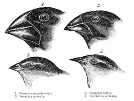
Selection

 

Recombination

Drift

Wright-Fisher model with alleles

Alleles can randomly fix or be lost through process called genetic drift

Wright-Fisher model showing the evolution of population of 10 genes over 16 generations. Allele variants are shown in white and black. Starting frequency black variant is 0.3.

(To avoid confusion: previously black was used to indicate parent, here black/white will refer to different alleles)

Enter allelic variants; we are looking at two alleles

Important: the fate of any allele under drift is to be lost or fixed, which ultimately means variation is lost (decays) with drift

Binomial process models allele sampling

We assume two alleles A, a, each with i and j=2N-i copies in generation t.

i=8, j=2\cdot 6-8=4

Let p_t=i/2N be the frequency of A in generation t, and q_t=1-p_t the frequency of a.

p_t = 8/12

p_{t+1} = 4/12

Prob(k A alleles in next generation) is \mathsf{Bin}(2N, \frac{i}{2N})

A more formal mathematical description goes as follows:

The sampling model for next generation t+1, given i A alleles in generation t, is

p_{t+1} = P(v_A=k) = {2N\choose k}\left( \frac{i}{2N} \right)^k \left(1 - \frac{i}{2N} \right)^{(2N - k)} = \mathsf{Bin}(2N, \frac{i}{2N})

NB: we here slightly change notation, with p_{t+1} = P(X=k). Also, we have omitted an index i in the expressions of p. The probability of observing k A alleles in generation t+1 will of course depend on the number i A alleles in the previous generation.

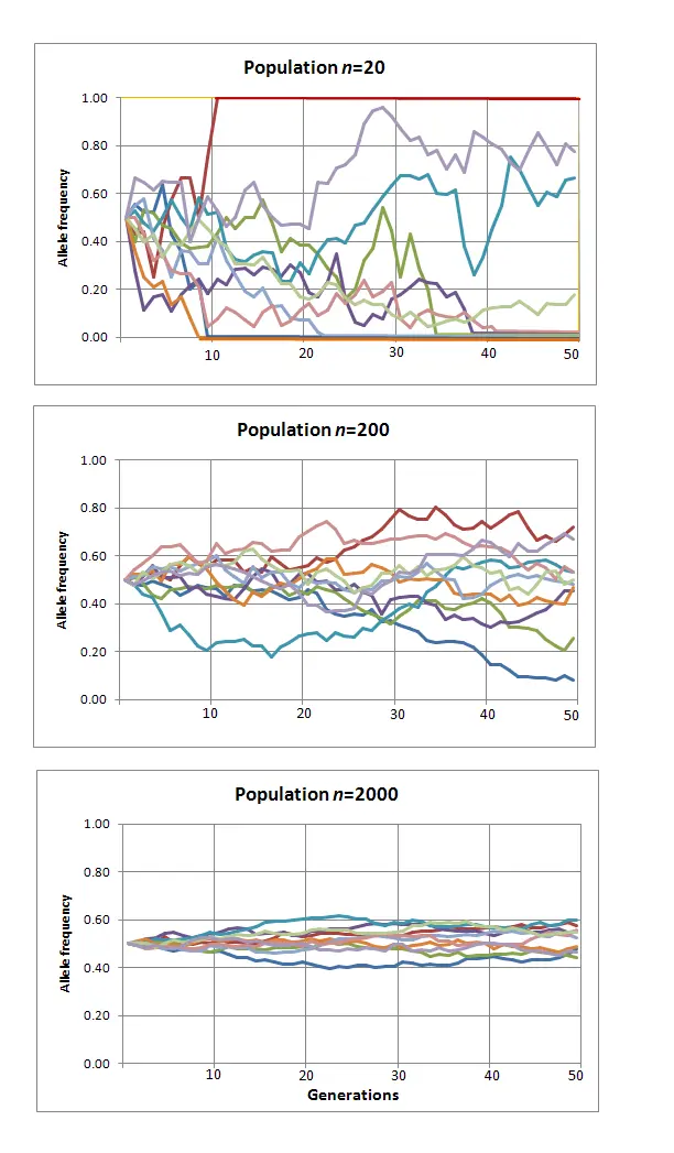
Genetic drift

To capture dynamics, follow allele frequency trajectory (p_t) as function of time.

##' Wright Fisher model - follow allele frequency distribution
##'
##' @param p0 Starting frequency
##' @param n Population size
##' @param generations Number of generations to simulate
##'
wright_fisher <- function(p0, n, generations) {
    x <- vector(mode = "numeric", length = generations)
    x[1] <- p0
    for (i in seq(2, length(x))) {
        x[i] <- rbinom(1, size = n, prob = x[i - 1])/n
    }
    x
}

# Example simulation and plot
set.seed(1223)
generations <- 100
n <- 100  # NB: haploid population size!
plot(1:generations, wright_fisher(0.5, n, generations), type = "l", ylab = "frequency",
    xlab = "generation", ylim = c(0, 1))

Figure 1: Genetic drift for different haploid(!) population sizes, starting frequency p_0=0.5. Note dependency of variance on population size N.

Mention neutral here as this is how alleles behave under drift: like gas particle diffusing up and down. Allele is eventually either fixed or lost.

Genetic drift

Figure 2: Genetic drift for different combinations of starting frequency and population size for n=50 repetitions per parameter combination. Note how variation and time to fixation depends on population size and starting frequency.

• fate of allele: fixation or loss \rightarrow eventually loss of variation
• probability of fixation \pi(p)=p, where p is the current frequency
• rate of drift (loss of variation) \propto \frac{1}{2N}

Simplifying assumptions -> rate of drift \propto \frac{1}{N} (\frac{1}{2N} in our treatment) (Leffler et al., 2012)

In reality population fluctuates and therefore Ne is substituted for N. Larger Ne -> smaller fluctuation in allele frequency (as evidenced in plots) -> maintain larger genetic diversity

Drift can be thought of as a force acting on a buoyant gas particle floating up and down at random.

Allele frequency distribution for N=1

Instead of looking at frequencies let’s switch to distributions of alleles for one individual, one locus. Then there are three possible genotypes (states) aa, aA, and AA. Let n=0,1,2 be an integer corresponding to each genotype (i.e., it counts the number of A alleles).

Assume individual mates with itself at random(!) starting in either of the three states. How does distribution evolve?

t=0

t=1

t=2

Example from (Gillespie, 2004, p. 24). We look at a single hermaphroditic individual that mates with itself at random. For each generation, given a genotype distribution, we calculate the outcome for the next generation. For instance, starting out in state 0 (only aa genotypes, hence only a alleles), we can only produce new aa genotypes and will therefore never leave state 0. The same holds for state 2. These states are absorbing states.

Starting from state 1 (aA) we can get aa genotype with 25% probability, since the probability of picking one a is 50%, and we perform two draws. Similarly, we get AA with 25% probability, leaving 50% to aA.

In the next generation, the aA genotype frequency is 0.5, to be split in fractions 0.25, 0.5, 0.25 as before, and so on.

To study the system we therefore need to enumerate the probabilistic outcomes from each state (aa -> 1, 0, 0, aA -> 0.25, 0.5, 0.25, AA <- 0, 0, 1). To get the state in next generation, we multiply the current distribution with these outcomes. The next slide gives Kimura’s example for the case where we have N=10 chromosomes.

Probability distributions of allele frequencies

Figure 3: Histogram showing the course of change of the allele frequency distribution with time (Kimura, 1983, Figure 3.4). When N large (\gtrsim 100) histogram can be approximated by continuous distribution (diffusion theory). Try recipe for different values of N.

Figure 4: Frequency distributions of the brown eye (bw^{75}) allele in replicate experimental populations (n\sim 100) of Drosophila melanogaster (8 , 8 ) (Buri, 1956)

Mathematical treatment of drift can become complicated: easier to study dynamics of heterozygosity

Kimura’s plot illustrates the allelic frequency distribution of replicate populations each consisting of N=10 sequences. There are two allelic types. The x axis corresponds to the proportion of populations in a given state (e.g., the y value for x=3/10 corresponds to the proportion of populations with 3 alleles of one type and 7 of the other). At t=0 all populations are in state 5/10.

Kimura’s plot is very instructive and students are encouraged to test the recipe code, increasing the number of states incrementally. For large enough N, the histograms can be approximated by continuous distributions. This observation led Kimura (even though diffusion equations were originally introduced to genetics by Fisher in 1922) to apply diffusion theory to obtain probability densities of allele frequencies, leading in turn to compact expressions of fixation probabilities, expected ages of alleles, and more. A treatment of diffusion theory is outside the scope of this course; the interested reader can consult e.g., (Ewens, 2004).

The Buri experiment is an empirical demonstration of Kimura’s plot.

On the sampling model, (Charlesworth & Charlesworth, 2010, p. 231) says:

It is, however, impossible to write down a simple algebraic expression for P, even without selection and mutation. [The equation] is useful for obtaining numerical results for relatively small populations, but becomes computationally demanding when N becomes very large.

Heterozygosity dynamics

Figure 5: Illustration of identity by descent (IBD) and state (IBS). Alleles in generation n are IBD but not IBS.

Let \mathcal{H}_t be the probability that two alleles are different by state. One can show that the time course evolution of \mathcal{H}_t in a randomly mating population consisting of N diploid hermaphroditic individuals is

\mathcal{H}_t = \mathcal{H}_0 \left( 1 - \frac{1}{2N} \right)^t

Important consequence: heterozygosity in WF population lost at rate 1/2N.

Alleles in generation n are IDB but not IBS

Motivation: mathematical description of genetic drift complicated for populations with more than one individual. Easier to study the evolution of heterozygosity.

Equation presented without details. Derivation in (Gillespie, 2004, pp. 25–27) starts from G=probability that two alleles are IBS

Heterozygosity dynamics

Figure 6: Plot of \mathcal{H}_t illustrating dependency on population size

Figure 7: Heterozygosity in black-footed ferret (Wisely et al., 2002). Example from Graham Coop (2020), Fig. 4.5

Example of how rapid decline in population size can affect heterozygosity.

Population size influences genetic diversity!

However, census population size not (always) the correct measure.

Dependency on population size: for large enough populations the decline will be very slow (drift speed ~ 1/2N)

Practical example shows loss of heterozygosity tell-tale signature of population decline; conversely, not easy to show population decline in large populations (e.g., marine species with large N_e) using heterozygosity as measure

(Barton et al., 2007, p. 369) “The relation between genetic diversity and population size is difficult to discern, in part, because it is extremely hard to estimate the numbers of most species and because the number that matters is an average back into the distant past”(!)

From (Graham Coop, 2020, p. 64)

To see how a decline in population size can affect levels of het- erozygosity, let’s consider the case of black-footed ferrets (Mustela nigripes). The black-footed ferret population has declined dramatically through the twentieth century due to destruction of their habitat and sylvatic plague. In 1979, when the last known black-footed ferret died in captivity, they were thought to be extinct. In 1981, a very small wild population was rediscovered (40 individuals), but in 1985 this population suffered a number of disease outbreaks. At that point of the 18 remaining wild individuals were brought into captivity, 7 of which reproduced. Thanks to intense captive breeding efforts and conservation work, a wild population of over 300 individuals has been established since. However, because all of these individuals are descended from those 7 individuals who survived the bottleneck, diversity levels remain low. Wisely et al. measured heterozygosity at a number of microsatellites in individuals from museum collections, showing the sharp drop in diversity as population sizes crashed (see Figure 4.5).

Segue: population size important; however, census population size is not always the measure we want when relating to genetic diversity

Effective population size

Assumptions underlying Wright-Fisher model seldom fulfilled for natural populations. In particular

• non-random mating (population structure)
• fluctuations of population census size

Therefore, magnitude of drift experienced by a population different from that predicted by population size

Technically correct definition (but see Waples (2022), Waples (2025)):

N_e is the size of an ideal population that would experience the same rate of genetic drift as the population in question.

ideal population: discrete generations with random mating, no evolutionary forces besides drift, no selective advantages

Mutation

Two-allele

Derive popgen stats

Finite sites

Recurrent mutations

Infinite alleles

Protein electrophoresis

Inifinite sites

DNA sequences

Mutations are generated randomly as changes in DNA. In WF model will be highlighted in black. We assume mutations are described by a Poisson process with rate \mu (per generation).

The mutation models are:

• two-allele model: used to derive popgen statistics
• finite sites model: recurrent mutations may occur, an assumption that is often omitted to facilitate calculations (e.g., coalescent)
• inifinite alleles model: every mutation leads to new allele (e.g., protein electrophoresis)
• infinite sites model: model commonly used for long DNA sequences

Additional model not presented here is the stepwise mutation model (mainly used to model repeats):

Mutation and drift

Genetic drift “moves” frequencies to the point that variation is lost via allele fixation or loss. New variation is introduced through mutation. We typically assume mutations are described by a Poisson process with rate \mu (per generation).

The mutation rate is denoted \mu, and the population scaled mutation rate is 2N_e\mu for haploid populations, 4N_e\mu for diploid, where N_e is the effective population size.

The mutation - drift balance is when the diversity lost due to drift equals the diversity gained due to mutation.

Figure 8: Variation is introduced by mutations (black) at rate \mu=1e^{-4} and is occasionally lost through genetic drift.

Segue: so if drift removes variation, what introduces it? Mutation!

Note that the mutation rate in the WF model is not meaningful; the value is simply chosen such that enough mutations show up in plot.

Tracing the evolution of mutations

Figure 9: Different mutations suffer different fates. Most mutations are lost in a couple of generations. Mutant alleles are colored black and their genealogies are highlighted with thicker edges.

Observation: most mutations are in fact lost

Recall: fixation probability \pi(p)=p

Difference to previous figure: here we highlight the genealogies

Mutation drift balance

Drift removes variation. Mutation reintroduces it. At equilibrium the change in variation by definition is 0. In terms of \mathcal{H}_t (the probability that two alleles are not identical by state), \Delta\mathcal{H}=0.

One can show¹ the classical formula that the equilibrium heterozygosity value is

\hat{\mathcal{H}} = \frac{4N_e\mu}{1 + 4N_e\mu}

\mu is often assumed known, and heterozygosity is easily calculated from data, which provides a way of estimating N_e.

The compound parameter 4N_e\mu is called the population scaled mutation rate and is commonly named \theta such that

\hat{\mathcal{H}} = \frac{\theta}{1 + \theta}

Gillespie (2004), pp. 30–31 uses a difference equation approach to derive \mathcal{H}. Briefly, he studies the time evolution of \mathcal{G}, the probability that two alleles drawn at random without replacement from the population are identical by state. Mutations are assumed unique, i.e., the infinite-alleles model. It holds

\mathcal{G}^\prime = (1-\mu)^2\left[ \frac{1}{2N} + \left( 1 - \frac{1}{2N} \right) \mathcal{G} \right]

where (1-\mu)^2 is the probability that no mutation occur in either of the two sampled alleles. Since \mu is small, (1-\mu)^2 \approx 1-2\mu, which after some manipulation gives the desired expression for \mathcal{H} = 1 - \mathcal{G}.

On pages 46–47, he shows that the expression for can be derived in a much simpler fashion using coalescent theory. Tracing two lineages backwards in time, the probability of coalescence is 1/2N, whereas the probability of a mutation is 1-(1-\mu)^2\approx 2\mu; \mathcal{H} is then simply the relative probability of the two events

\mathcal{H} = \frac{2\mu}{2\mu + 1/2N} = \frac{4N\mu}{4N\mu + 1}

1. see (Gillespie, 2004, p. 29 – 31) for a concise treatement

The neutral theory of evolution

Mutation drift balance, together with the observation during 50’s-60’s that polymorphism was more common than expected, is the foundation of the neutral theory of evolution (Kimura, 1983): allele frequencies may change and fix due to chance alone and not selection; most mutations behave as if they are neutral.

Nearly neutral theory (Ohta, 1973) was later developed to explain failure to predict scaling of polymorphism with population size: most mutations are not neutral but slightly deleterious and purged from population by natural selection.

Figure 10: Heterozygosity H=\frac{\theta}{1 + \theta} predicted by the neutral theory. Shaded region shows typical heterozygosities in animals (y-axis). The observed N_e\mu range is higher than predicted from plot. From Hurst (2009), Fig 1.

Related to rate of substitution and molecular evolution is the work of Kimura that lead to the development of the neutral theory.

Motivation: if polymorphic sites deleterious, should not expect much polymorphism.

Low levels of polymorphism expected assuming little balancing selection (Hurst, 2009, p. 87); however electrophoretic studies showed polymorphism common. Would lead to detrimental load (Kimura & Ohta, 1971) -> therefore majority of polymorphism must evolve neutrally (dynamics). Also: rate of evolution (on protein level) too high (Haldane’s dilemma)

On the shaded region: the observed range of N_e\mu is larger than that which is predicted by the plot, and since \mu is constrained within a couple of orders of magnitude, N_e must vary more than predicted by the (strictly) neutral theory.

Conversely: given a constrained \mu, we observe a range of N_e\mu that predicts a heterozygosity range H, which is much larger than that which we observe. In other words, the heterozygosity range is much lower than predicted by the neutral, given the observed N_e\mu range, so some other process must reduce variation somehow.

The general idea of nearly neutral theory is that most mutations are slightly deleterious and therefore purged by natural selection, thereby reducing observed variation. The efficacy of purging depends in turn on the effective population size, such that species with small N_e will have a harder time getting rid of potentially damaging variants.

Mutation rate can be estimated from substitution rate

Mutation enters populations and may be fixed by drift. Therefore, with time there will be fixed differences, or substitions (typically in the evolution of species) between populations, or species. In molecular evolution, the substition rate, \rho, is the most interesting quantity.

The total number of new mutations in every generation is 2N\mu (total number of gametes times mutation rate)

New mutations fix at a rate 1/2N

Therefore, the average rate of substitution, \rho, is 2N\mu\times1/2N, or

\rho=\mu

which is independent of population size!

Practical implication: we can estimate mutation rate from the substitution rate at neutrally evolving sites (e.g., Kumar & Subramanian (2002))

What happens when sufficient amount of time passes? Mutations fix and generate substitutions between species. This slide presents Kimura’s remarkable result regarding mutation rate and substitution rate!

On 2N\mu: the larger the population, the larger the number of mutations that can fix

If 4N\mu>>0 no new mutations can fix. Issue here is there is no explicit mention of DNA sequence -> introduction of infinite sites model

For practical note on estimation of mutation rate see e.g., (Hubisz & Siepel, 2020, p. 247)

(Kumar & Subramanian, 2002, first paragraph):

Rates of point mutation can be determined indirectly by estimating the rate at which the neutral substitutions accumulate in protein-coding genes

Bibliography

Barton, N. H., Briggs, D. E. G., Eisen, J. A., Goldstein, D. B., & Patel, N. H. (2007). Evolution. Cold Spring Harbor Laboratory Press.

Buri, P. (1956). Gene Frequency in Small Populations of Mutant Drosophila. Evolution, 10(4), 367–402. https://doi.org/10.1111/j.1558-5646.1956.tb02864.x

Charlesworth, B., & Charlesworth, D. (2010). Elements of Evolutionary Genetics. Roberts and Company Publishers.

Ewens, W. J. (2004). Mathematical Population Genetics (S. S. Antman, J. E. Marsden, L. Sirovich, & S. Wiggins, Eds.; Vol. 27). Springer. https://doi.org/10.1007/978-0-387-21822-9

Gillespie, J. H. (2004). Population Genetics: A Concise Guide (2nd edition). Johns Hopkins University Press.

Graham Coop. (2020). Notes on Population Genetics. https://github.com/cooplab/popgen-notes

Hubisz, M., & Siepel, A. (2020). Inference of Ancestral Recombination Graphs Using ARGweaver. In J. Y. Dutheil (Ed.), Statistical Population Genomics (pp. 231–266). Springer US. https://doi.org/10.1007/978-1-0716-0199-0_10

Hurst, L. D. (2009). Genetics and the understanding of selection. Nature Reviews Genetics, 10(2), 83–93. https://doi.org/10.1038/nrg2506

Kimura, M. (1983). The neutral theory of molecular evolution. Cambridge University Press. https://doi.org/10.1017/CBO9780511623486

Kimura, M., & Ohta, T. (1971). Protein Polymorphism as a Phase of Molecular Evolution. Nature, 229(5285), 467–469. https://doi.org/10.1038/229467a0

Kumar, S., & Subramanian, S. (2002). Mutation rates in mammalian genomes. Proceedings of the National Academy of Sciences, 99(2), 803–808. https://doi.org/10.1073/pnas.022629899

Leffler, E. M., Bullaughey, K., Matute, D. R., Meyer, W. K., Ségurel, L., Venkat, A., Andolfatto, P., & Przeworski, M. (2012). Revisiting an Old Riddle: What Determines Genetic Diversity Levels within Species? PLOS Biology, 10(9), e1001388. https://doi.org/10.1371/journal.pbio.1001388

Ohta, T. (1973). Slightly Deleterious Mutant Substitutions in Evolution. Nature, 246(5428), 96. https://doi.org/10.1038/246096a0

Waples, R. S. (2022). What Is Ne, Anyway? Journal of Heredity, 113(4), 371–379. https://doi.org/10.1093/jhered/esac023

Waples, R. S. (2025). The Idiot’s Guide to Effective Population Size. Molecular Ecology, e17670. https://doi.org/10.1111/mec.17670

Wisely, S. M., Buskirk, S. W., Fleming, M. A., McDonald, D. B., & Ostrander, E. A. (2002). Genetic Diversity and Fitness in Black-Footed Ferrets Before and During a Bottleneck. Journal of Heredity, 93(4), 231–237. https://doi.org/10.1093/jhered/93.4.231