
Principal component analysis
Clustering and dimensionality reduction
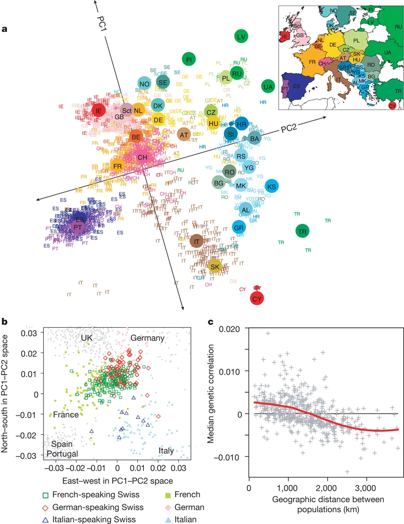
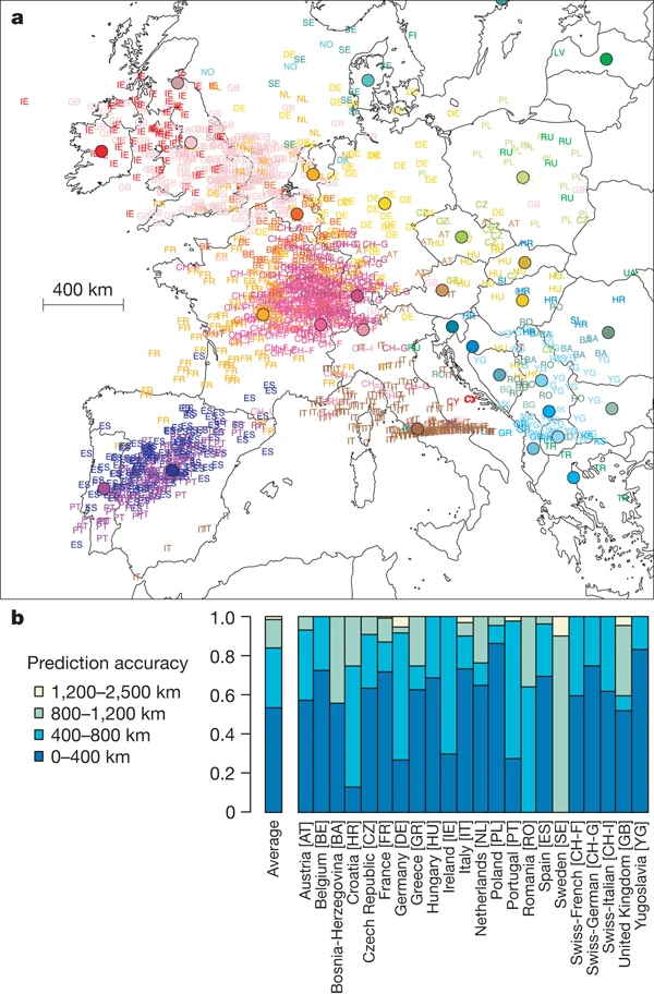
PCA in population genetics

Beware: Novembre & Stephens (2008) pointed out that patterns may be due to mathematical artifacts and not necessarily directly inform us about the underlying demographic process!
PCA in population genetics
PCA is a matrix factorization technique
An entry in the genotype matrix is approximated by the K first loadings
G_{ij} \approx \mathbf{\Lambda}_i \mathbf{F}_j
Toy example of PCA for population genetics
gen <- t(matrix(c(1, 0, 2, 0, 2, 0, 2, 1, 1, 1, 0, 1, 0, 2, 1, 2, 1, 1, 1, 1, 1,
    0, 1, 0, 2, 0, 1, 1, 0, 2, 1, 2, 0, 1, 0), 5, by = TRUE))
colnames(gen) <- paste0("Ind", 1:5)
rownames(gen) <- paste0("SNP", 1:7)
print(gen)
Ind1 Ind2 Ind3 Ind4 Ind5
SNP1 1 1 1 0 0
SNP2 0 1 2 1 2
SNP3 2 1 1 0 1
SNP4 0 0 1 2 2
SNP5 2 1 1 0 0
SNP6 0 0 1 1 1
SNP7 2 2 1 1 0

Idea: project the data into a low dimensional space that explains the largest amount of variance
Geometric interpretation

Variance maximization and eigen value decomposition
- Collapse p features (p>>n) to few latent features and keep variation
- Rotation and shift of coordinate system toward maximal variance
- PCA is an eigen matrix decomposition problem
Example of PCA plot of Monkeyflower data
We will use plink2 (Chang et al., 2015) to generate PCA plots.
LD pruning
PCA assumes independent markers!
PCA
Construct PCA from subset of pruned markers

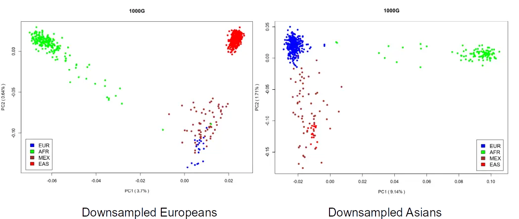
Uneven sampling may distort PCA projections
“The results described here provide an explanation. First, from Equation 10 it can be seen that the matrix M is influenced by the relative sample size from each population through the components t_i. For instance, even if all populations are equally divergent from each other, those for which there are fewer samples will have larger values of t_i because relatively more pairwise comparisons are between populations.”
M=XX^T=\frac{1}{N}\sum_{ij}x_ix_j N=N_{pop1}+N_{pop2}+N_{pop3}+...=\sum_k N_k M_{uneven}=\sum_{ijk}\frac{1}{N_k}x_{ik}x_{jk}
- Potential solution: normalize each sample by its population size before computing the covariance matrix.
- Is it still an unsupervised technique?
Example of uneven sampling
Bibliography
Cavalli-Sforza, L. L., & Edwards, A. W. F. (1967). Phylogenetic analysis. Models and estimation procedures. American Journal of Human Genetics, 19(3 Pt 1), 233–257.
Chang, C. C., Chow, C. C., Tellier, L. C., Vattikuti, S., Purcell, S. M., & Lee, J. J. (2015). Second-generation PLINK: Rising to the challenge of larger and richer datasets. GigaScience, 4(1), s13742-015-0047-8. https://doi.org/10.1186/s13742-015-0047-8
McVean, G. (2009). A Genealogical Interpretation of Principal Components Analysis. PLOS Genetics, 5(10), e1000686. https://doi.org/10.1371/journal.pgen.1000686
Menozzi, P., Piazza, A., & Cavalli-Sforza, L. (1978). Synthetic Maps of Human Gene Frequencies in Europeans. Science, 201(4358), 786–792. https://doi.org/10.1126/science.356262
Novembre, J., Johnson, T., Bryc, K., Kutalik, Z., Boyko, A. R., Auton, A., Indap, A., King, K. S., Bergmann, S., Nelson, M. R., Stephens, M., & Bustamante, C. D. (2008). Genes mirror geography within Europe. Nature, 456(7218), 98–101. https://doi.org/10.1038/nature07331
Novembre, J., & Stephens, M. (2008). Interpreting principal component analyses of spatial population genetic variation. Nature Genetics, 40(5), 646–649. https://doi.org/10.1038/ng.139
Pritchard, J. K. (n.d.). An Owner’s Guide to the Human Genome. Retrieved August 18, 2025, from https://web.stanford.edu/group/pritchardlab/HGbook.html