Investigating the diversity landscape in Monkeyflower
Author
Per Unneberg
Published
18-Sep-2025
About
In this exercise we will look at measures that describe variation and compile statistics along a sequence. By scanning variation in windows along the sequence (a.k.a. genomic scan) we can identify outlier regions whose pattern of variation could potentially be attributed to causes other than neutral processes, such as adaptation or migration. We will use the Monkeyflower system to generate a diversity landscape.
Commands have been run on a subset of the data
The commands of this document have been run on a subset (a subregion) of the data. Therefore, although you will use the same commands, your results will differ from those presented here.
Learning objectives
describe and calculate commonly used measures of variation, including nucleotide diversity \(\pi\), divergence \(d_{XY}\) and differentiation \(F_{ST}\)
perform genome scans of diversity and plot the results
Choose one of Modules and Virtual environment to access relevant tools.
Modules
Execute the following command to load modules:
# NB: the following tools are not available as modules:
# - csvtk
module load bioinfo-tools \
    bcftools/1.20 bedtools/2.31.0 pixy/1.2.5.beta1 \
    vcftools/0.1.16
Virtual environment
Run the pgip initialization script and activate the pgip default environment:
source /cfs/klemming/projects/supr/pgip_2025/init.sh# Now obsolete!# pgip_activate
Then activate the full environment:
# pgip_shell calls pixi shell -e full --as-ispgip_shell
Copy the contents to a file pixi.toml in directory genetic-diversity, cd to directory and activate environment with pixi shell:
Some of the programs require we prepare population files. For pixy, this is a headerless, tab-separated file with sample and population columns. The sampleinfo.csv file contains the information we need; the sample names have been prefixed with a three-letter code to indicate population (apart from ssp. puniceus which also comes with a single letter R or Y indicating ecotype). Table 2 summarizes the populations and samples.
Code
# R code to generate sample population summarydata<-tibble(read.csv("sampleinfo.csv"))data<-data%>%mutate(Population =SampleAlias)%>%mutate(across(.col ="Population", .names ="Population", .fns =list(~str_replace(.x,"(.+)-.+$", "\\1"))))%>%mutate(across(.col ="Population", .names ="Population", .fns =list(~str_replace(.x,"(CLV)_.+", "\\1"))))data%>%group_by(Population, ScientificName)%>%summarise(n =n(), samples =paste(SampleAlias, collapse =", "))%>%kable()
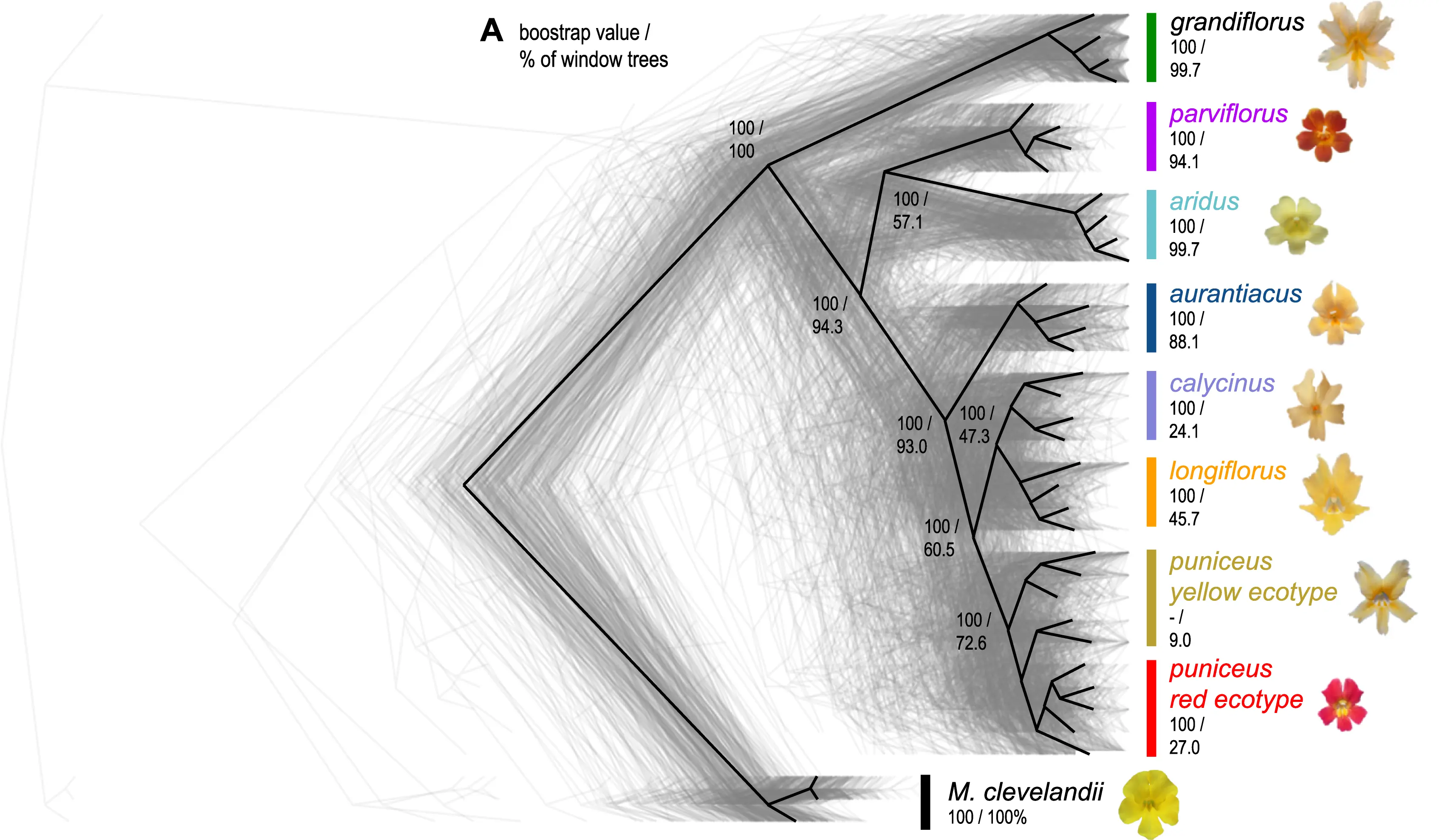
Figure 1: Evolutionary relationships across the radiation
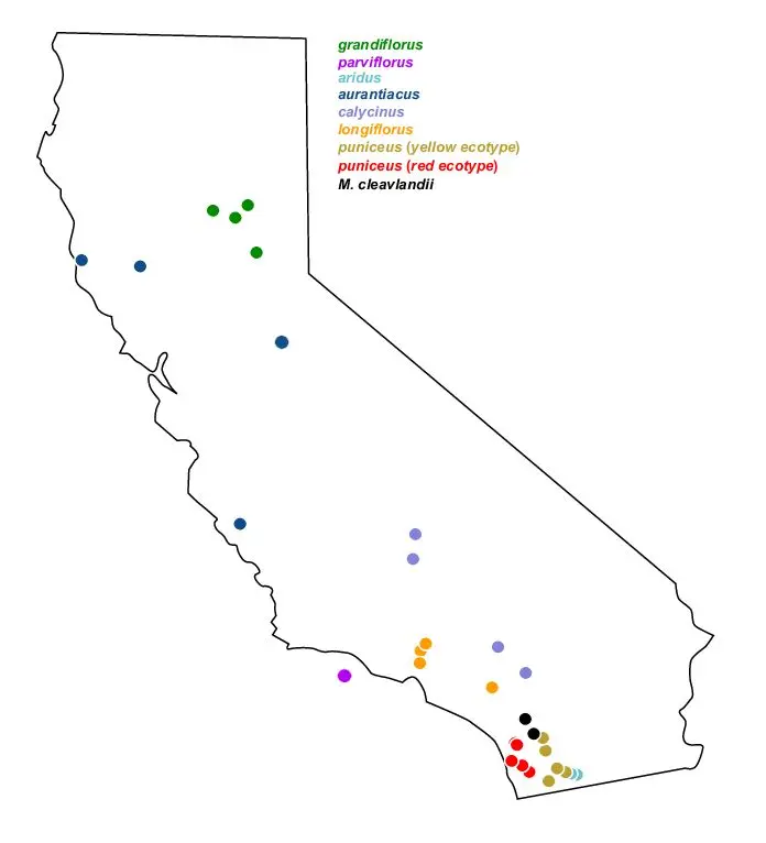
Figure 2: Monkeyflower sampling locations
We convert the sample information with csvtk. We also add a populations file with all samples belonging to the same population:1
csvtk mutate --name Population --fields SampleAlias sampleinfo.csv |csvtk cut --fields SampleAlias,Population |csvtk replace --fields Population --pattern"(.+)-.+$"--replacement"\$1"|csvtk replace --fields Population --pattern"(CLV)_.+"--replacement"\$1"|csvtk del-header --out-tabs> populations.txtcsvtk cut --fields SampleAlias sampleinfo.csv |csvtk mutate --name Population --fields SampleAlias |csvtk replace --fields Population --pattern".+"--replacement"ALL"|csvtk del-header --out-tabs> populations.ALL.txt
vcftools, on the other hand, requires that populations are specified as separate files, containing the individuals of each population. We can use the populations.txt file to quickly generate population-specific files, and we add an ALL population, treating all samples as coming from the same population:
for pop in ARI AUR CAL CLV GRA LON PAR PUN-R PUN-Y;docsvtk--no-header-row grep --tabs--fields 2 --pattern"$pop" populations.txt |\csvtk cut --tabs--fields 1 >$pop.txt;donecsvtk cut --tabs--no-header-row--fields 1 populations.txt > ALL.txt
We define environment variables to make the downstream commands easier to type:
VCF=allsites.vcf.gzPOPS=populations.txt
Generating and visualising diversity statistics
Compiling statistics with vcftools
Create an output directory for the results and define some environment variables:
mkdir-p 01-vcftoolsOUT=01-vcftools/allsites
Nucleotide diversity (\(\pi\))
Nucleotide diversity can be calculated by site (--site-pi) or in windows (--window-pi)2.
# Set your window size higher, e.g., 10kbvcftools--gzvcf$VCF--window-pi 1000 --out$OUT2> /dev/null
On genome scans and window sizes
Genetic diversity estimates can be noisy, so we often want to compute values in sliding windows across a sequence. Choosing window size can be as simple as trying out different values, often ranging from single to several hundred kilobases. As always, the appropriate size depends on the analyses.
One rule of thumb that can be applied is that the window size should be larger than the genomic background of linkage disequilibrium (LD). Recall, LD is the non-random co-segregation of alleles at two or more loci. Linked loci will induce correlations in window-based statistics, so by choosing a window size larger than the LD background, we ensure that our windows are, in some sense, independent.
For this reason, a common approach is to calculate some measure of LD between marker pairs, and generate a plot of LD decay. This is outside the scope of this exercise, but the interested reader can consult the plink documentation for ways to do this. See also Figure 3 for an example plot.
Figure 3: Properties of genetic variation and inferred demographic history in sampled A. millepora. Fuller et al. (2020), Figure 2. Upper left plot illustrates LD as a function of physical distance. Here, choosing a window size 20-30kb would ensure that most windows are independent.
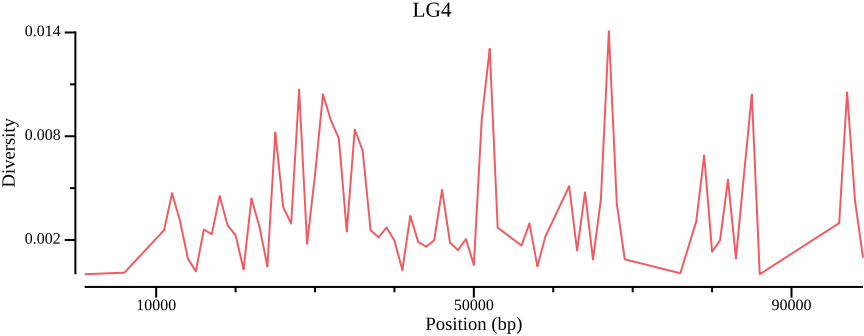
Even though single point summary statistics can be informative, we can get an overview of the distribution over the chromosome by plotting:
csvtk plot line --tabs$OUT.windowed.pi -x BIN_START -y PI \--point-size 0.01 --xlab"Position (bp)"\--ylab"Diversity"--title LG4 --width 9.0 --height 3.5 \>$OUT.png
Figure 4: Nucleotide diversity across LG4 for all populations.
Figure 4 shows the diversity for all populations. We would also be interested in comparing the diversity for different populations. This can be achieved by passing a population file to bcftools view and piping (|) the output to vcftools:
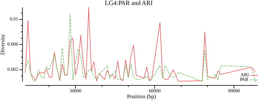
With some csvtk magic we can combine the measures and plot:
# When assigning a constant must enclose it in single quotes within double quotescsvtk mutate2 --tabs--name Population --expression" 'ARI' "\$OUT.ARI.windowed.pi >$OUT.ARI.wpicsvtk mutate2 --tabs--name Population --expression" 'PAR' "\$OUT.PAR.windowed.pi >$OUT.PAR.wpicsvtk concat --tabs$OUT.ARI.wpi $OUT.PAR.wpi |\csvtk plot --tabs line --x BIN_START -y PI \--group-field Population \--point-size 0.01 --xlab"Position (bp)"\--ylab"Diversity"--title"LG4:PAR and ARI"\--width 9.0 --height 3.5 \>$OUT.ARI.PAR.png 2>/dev/null
Figure 5: Nucleotide diversity across LG4 comparing populations ARI and PAR.
\(F_{ST}\)
Since \(F_{ST}\) is a statistic that compares populations, we must supply two or more of the population files we defined above. A population file name is passed to the --weir-fst-pop option. Calculations are done by site per default, but let’s calculate \(F_{ST}\) for a comparison of two populations in 100kb windows:
# Set your window size higher, e.g., 100000vcftools--gzvcf$VCF--weir-fst-pop ARI.txt \--weir-fst-pop PAR.txt \--fst-window-size 1000 \--out$OUT.ARI-PAR
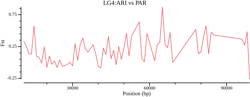
csvtk plot line --tabs$OUT.ARI-PAR.windowed.weir.fst \-x BIN_START -y MEAN_FST \--point-size 0.01 --xlab"Position (bp)"\--ylab"Fst"--title"LG4:ARI vs PAR"\--width 9.0 --height 3.5 \>$OUT.ARI-PAR.windowed.weir.fst.mean.png
Figure 6: Mean \(F_{ST}\) across LG4, comparing ARI and PAR populations.
Compiling statistics with pixy
The vcftools statistics that we just calculated have a couple of issues:
they have been calculated on unfiltered data; this can be somewhat remediated by applying a depth-based filter
a more concerning problem is that even if we did apply a filter, all missing sites would be treated as invariant sites, when in reality the windows would need to be adjusted to the number of accessible sites within a window. This number could be calculated from a mask file, but adds some complexity to the calculations.
Instead of applying filters, let’s first try out an alternative solution. pixy is a program that facilitates the calculation of nucleotide diversity within \(\pi\) and between \(d_{XY}\) populations from a VCF, as well as differentiation (\(F_{ST}\)). It also takes invariant sites and missing data into consideration. Another nice feature is that by providing a population file with all samples, every population comparison is done on the fly, so only one run is needed!
Calculating per-site statistics takes too long time, so we will only generate windowed output here. This may still take a couple of minutes though.
mkdir-p 02-pixy# Set your window size higher, e.g., 100kbpixy--stats pi fst dxy \--vcf$VCF\--populations populations.txt \--window_size 1000 \--output_folder 02-pixy \--n_cores 4
For windowed output, the pixy output files contain information on the windows, the number of missing sites, number of snps, and more. The first column corresponds to the population, which means we can easily select lines matching population(s) of interest. For a full description, consult the documentation. Note that because we provided a population file defining two populations, diversity is calculated per population.
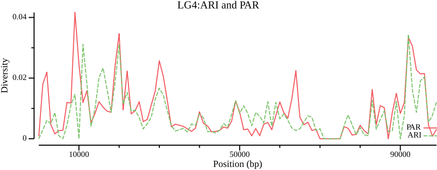
We conclude by plotting diversity for ARI and PAR
# Possibly remove NA values that otherwise would throw errorcsvtk filter2 --tabs\--filter'$avg_pi != "NA" && ($pop == "ARI" || $pop == "PAR") '\ 02-pixy/pixy_pi.txt |\csvtk plot line --tabs--x window_pos_1 -y avg_pi \--group-field pop \--point-size 0.01 --xlab"Position (bp)"\--ylab"Diversity"--title"LG4:ARI and PAR"\--width 9.0 --height 3.5 \> 02-pixy/pixy_pi.ARI-PAR.txt.png
Figure 7: Mean diversity across LG4 for ARI and PAR.
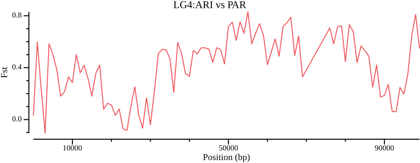
Figure 8: Mean \(F_{ST}\) across LG4 for ARI vs PAR.
Comparing Figure 8 to Figure 6 shows a stark contrast, so clearly, how you filter and handle invariant/missing data will strongly affect the outcome.
OPTIONAL: Apply filters to pixy and vcftools output and compare
Generate depth filters, utilizing the knowledge from the variant filtering lab, and apply them to the VCF file. Rerun a couple of pixy and vcftools stats to see how it affects the outcome. Provided you use identical window sizes, you could make a scatter plot of a statistic of the two tools against oneanother.
Genome scans and genomic features
Working with Z-transformed data
Transforming raw data to Z-scores can facilitate the scan for outlier regions. However, there is no easy way to do this with csvtk, so here is some template R code to do this from pixy data.
pi<-read.table("pixy_pi.txt", header =TRUE)# Select population PARdata<-data[data$pop=="PAR", ]x<-data$avg_piz<-(x-mean(x, na.rm =TRUE))/sd(x, na.rm =TRUE)# Plot data along chromosome and identify region by eye plot(x =# data$window_pos_1, y = z, xlab = 'Position (bp)')
Stratifying by genomic feature
pixy accepts as input a BED file that defines coordinates of genome features. Here is an example of how to extract CDS regions and then compile results with pixy:
pixy--vcf allsites.vcf.gz --stats pi \--populations populations.txt \--output_prefix cds --bed_file CDS.bed
Monkeyflower diversity landscape
Drawing on what you learned earlier today about filtering, and with the help of the command examples above, you can now start exploring the Monkeyflower diversity landscape. Try different population comparisons, perform outlier analyses, and see if you can find candidate regions of interest. If you want inspiration, take a look at the methods section of Stankowski et al. (2019).
Here are some suggested actions that you can take, but feel free to look at the data in any way you want.
Apply depth filter to VCF
Create a VCF subset of all samples and generate a depth filter, following the guidelines in the filtering exercise.
Run an outlier analysis and investigate significant loci
Z-transform a statistic and try to identify outliers. You can compare the coordinates of any significant locus with those in the provided annotation file MAUR_annotation_functional_submission.gff.
Compile data by genome feature
Use the annotation file MAUR_annotation_functional_submission.gff to generate BED files that define the regions of some features of interest, e.g., genes, introns, or UTRs. Do the results make sense?
Reproduce distributions of diversity statistics for different population comparisons
Danecek, P., Auton, A., Abecasis, G., Albers, C. A., Banks, E., DePristo, M. A., Handsaker, R. E., Lunter, G., Marth, G. T., Sherry, S. T., McVean, G., & Durbin, R. (2011). The variant call format and VCFtools. Bioinformatics (Oxford, England), 27(15), 2156–2158. https://doi.org/10.1093/bioinformatics/btr330
Danecek, P., Bonfield, J. K., Liddle, J., Marshall, J., Ohan, V., Pollard, M. O., Whitwham, A., Keane, T., McCarthy, S. A., Davies, R. M., & Li, H. (2021). Twelve years of SAMtools and BCFtools. GigaScience, 10(2), giab008. https://doi.org/10.1093/gigascience/giab008
Fuller, Z. L., Mocellin, V. J. L., Morris, L. A., Cantin, N., Shepherd, J., Sarre, L., Peng, J., Liao, Y., Pickrell, J., Andolfatto, P., Matz, M., Bay, L. K., & Przeworski, M. (2020). Population genetics of the coral Acropora millepora: Toward genomic prediction of bleaching. Science, 369(6501), eaba4674. https://doi.org/10.1126/science.aba4674
Korunes, K. L., & Samuk, K. (2021). Pixy: Unbiased estimation of nucleotide diversity and divergence in the presence of missing data. Molecular Ecology Resources, 21(4), 1359–1368. https://doi.org/10.1111/1755-0998.13326
Quinlan, A. R., & Hall, I. M. (2010). BEDTools: A flexible suite of utilities for comparing genomic features. Bioinformatics, 26(6), 841–842. https://doi.org/10.1093/bioinformatics/btq033
Stankowski, S., Chase, M. A., Fuiten, A. M., Rodrigues, M. F., Ralph, P. L., & Streisfeld, M. A. (2019). Widespread selection and gene flow shape the genomic landscape during a radiation of monkeyflowers. PLOS Biology, 17(7), e3000391. https://doi.org/10.1371/journal.pbio.3000391
Footnotes
Whenever you see a large number of commands strung together with pipe (|) characters and you are unsure what is going on, I suggest you build the command from scratch, one statement at a time. So, begin with csvtk mutate up until the first pipe character, and once you understand what is going on, add the next statement up until the next pipe character, and so on.↩︎
Recall; the dataset used to render these pages is much smaller, which is why we use a smaller window size below. Consequently, your plot will look different.↩︎