Alleles and genealogies

More descriptions of genetic data

Per Unneberg

Alleles as algebraic entities

Recall: alleles refer to different variants of a sequence at a locus (genomic position).

Whatever the underlying molecular nature (gene, chromosome, nucleotide, protein), let’s represent a locus by a letter, e.g., A (B if two loci, and so on)

If locus has many alleles 1, 2, ... , could use indexing A_1, A_2, ....

Will use combination A, a for bi-allelic loci from now on

Example: gene coding for flower color

A red color

a white color

Punnett square

\

A

a

A

a

Genotype

aa

Aa

AA

Phenotype

Heterozygote has intermediate color phenotype (pink).

Until now the examples have been based on nucleotide sequences. However, much of population genetic theory was developed before the nature of heredity (DNA) was known. In these early days, an allele would refer to variant forms of a gene, observed as differences in phenotypes. Genes, or loci, would be denoted using alphabetic characters, such as A, and allelic types could be referenced with indices, e.g., A_1, A_2, ..., A_n.

To simplify calculations, we often look at one locus and we assume two alleles, whereby we skip the indices and denote the allelic pairs A and a (although note that notations differs from author to author; for instance Gillespie (2004) uses A_1, A_2 for bi-allelic loci). For two-locus systems we simply denote the second allele with B, b, and so on.

The example shows a hypothetical locus having two alleles A and a that have phenotypes red and white flower color, and where heterozygotes are colored pink. The Punnett square shows how gamete combinations form genotypes and their corresponding phenotypes.

Alleles and frequencies

We will be interested in looking at the dynamics of alleles, i.e., how their abundances in the population change over time. Therefore we want to measure the frequencies of alleles A and a.

Example

Assume following population (n=10, with n_{AA}=5, n_{Aa}=4, n_{aa}=1):

Let p be frequency of A alleles, q=1-p frequency of a alleles; then

5 AA individuals, 4 Aa individuals \Rightarrow p=\frac{5\cdot2 + 4\cdot1}{10\cdot2}=\frac{14}{20}=0.7

and q=1-p=\frac{6}{20}=0.3

Inserting frequencies into Punnett square gives expected frequency of offspring genotypes.

\

A (p=0.7)

a (q=0.3)

A (p=0.7)

p\cdot p = 0.49

p\cdot q = 0.21

a (q=0.3)

q\cdot p = 0.21

q\cdot q = 0.09

Expected allele frequencies after mating: p=p^2 + pq=0.7, q=1-p=0.3

Given n diploid individuals, there are 2n alleles in the population. The frequency of allele A is then the homozygote AA times two, plus one times the individuals carrying one A.

The Punnett square shows that the expected homozygote frequencies are 0.49 and 0.09 for AA and aa, and hence, the frequency of Aa is 1 - 0.49 - 0.09 = 0.42 = 0.21 + 0.21 = 2pq

In absence of evolutionary forces alleles are in equilibrium

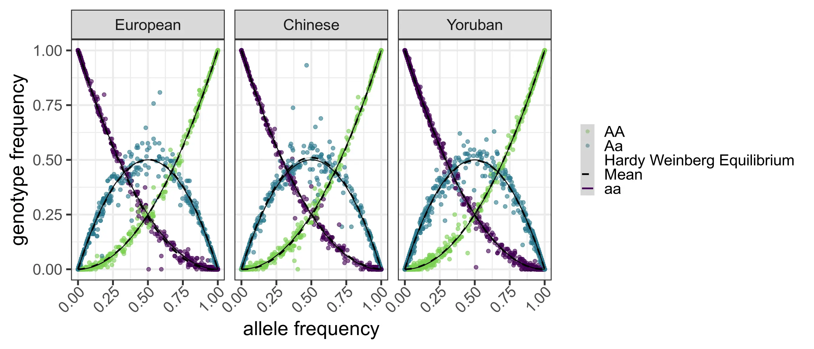
The Hardy-Weinberg equilibrium

For a locus, let A and a be two different alleles and let p be the frequency of the A allele and q=1-p the frequency of the a allele. In the absence of mutation, drift, migration, and other evolutionary processes, the equilibrium state is given by the Hardy-Weinberg equilibrium (HWE).

	A (p)	a (q)
A (p)	p^2	pq
a (q)	qp	q^2

Genotype:	AA	Aa	aa
Frequency:	p^2	2pq	q^2
	f_{AA}	f_{Aa}	f_{aa}

HWE assumption

Under HWE assumption, neither allele nor genotype frequencies change over time.

Importantly, we can calculate allele frequencies from genotype frequencies and vice versa.

p = f_{AA} + \frac{f_{Aa}}{2} = p^2 + pq\\ q = f_{aa} + \frac{f_{Aa}}{2} = q^2 + pq\\

Segue: apart from describing the variation via e.g., diversity measures, we want to model how allele frequencies change in time. As (Gillespie, 2004, preface p. xi) points out, “While genotype frequencies are easily measured, their change is not”

IOW: describing variation fine, but where does it come from and how does it change?

If assumptions of HWE hold, we have no change of variation. However, we want to look at change of variation and disentangle the forces that impose change

HWE assumption gives us a way to calculate allele frequencies from genotype frequencies. How well do these assumptions hold in real data? See next slide.

Natural populations do mate randomly?

Figure 1: Hardy-Weinberg proportions in 10,000 SNPs on chromosome 22 from three populations based on 1000 genomes data. For each SNP, genotypes are given as counts (minor/heterozygote/major), converted to frequencies and plotted on the y-axis. Allele frequencies are obtained from genotype frequencies and plotted on the x-axis. Most observations follow HWE proportions. Deviations from HWE can indicate sample QC issues, or that there is population structure. Illustration inspired by cooplab (2011).

So how do the HWE assumptions hold up in real data? The figure shows three human populations from the 1000 genomes data, for which 10,000 SNPs have been selected. For each SNP, we know the genotype frequencies AA, Aa, aa and can therefore calculate the allele frequencies for A and a using the equations on the preceding slide (e.g., p=p_{AA}+p_{Aa}/2).

Note that 1000 genomes data have sorted genotype frequencies, so to produce nice symmetrical plots, half the genotype frequencies have been reversed (minor/het/major -> major/het/minor).

See https://stackoverflow.com/questions/26587940/ggplot2-different-legend-symbols-for-points-and-lines for legend customization.

The Wahlund effect and population substructure

Population P1

p_A = 1 \Rightarrow p_A^2 = 1, p_a^2=2p_Ap_a=0

Population P1

p_a = 1 \Rightarrow p_a^2 = 1, p_A^2=2p_Ap_a=0

Both subpopulations are in HWE!

Population P1+P2:

p_A=p_a=0.5 so we would expect 50% heterozygotes - but there are none!

This is known as the Wahlund effect where the loss of heterozygosity is due to population substructure.

Summarising allele frequencies

Going back to the DNA example let’s tabulate the minor allele frequencies (MAFs):

	1	2	3	4	5	6	7	8	9	10	11	12	13	14	15
	T	T	A	C	A	A	T	C	C	G	A	T	C	G	T
	T	T	A	C	G	A	T	G	C	G	C	T	C	G	T
	T	C	A	C	A	A	T	G	C	G	A	T	G	G	A
	T	T	A	C	G	A	T	G	C	G	C	T	C	G	T
MAF	0	1	0	0	2	0	0	1	0	0	2	0	1	0	1

Site-frequency spectrum (SFS)

We can count all the different frequency classes {x_0, x_1, x_2, ...} and make a frequency table or plot it:

Genealogies and mutations

Assuming we know how the samples are related and we know the ancestral sequence, we can plot the mutations (circles) on a genealogy.

Note the correspondence between frequency classes in the SFS and number of samples below a mutation.

The obsession of population genetics

Population genetics is about (Gillespie, 2004)

1. describing the genetic structure of populations
2. constructing theories on the forces that influence genetic variation

Questions to ponder:

• why does variation look the way it does?
• how is variation maintained?
• how does variation change over time (\Delta p)?
• what forces shape the genetic structure of populations?

p=0.1

\large\rightarrow

p=0.5

\large\rightarrow

p=0.9

From HWE: we want to look a the creation, maintenance and loss of variation and what forces affect it

Goal: describe theory behind evolving populations. This has been an obsession for a long time, even before DNA was known. We need to get back to basics.

Bibliography

cooplab. (2011). Population genetics course resources: Hardy-Weinberg Eq. In gcbias. https://gcbias.org/2011/10/13/population-genetics-course-resources-hardy-weinberg-eq/

Gillespie, J. H. (2004). Population Genetics: A Concise Guide (2nd edition). Johns Hopkins University Press.