
The Wright-Fisher model
Of population models and genealogies
Wright-Fisher model
Model of populations that describes genealogical relationships of genes (chromosomes) in a population under the following assumptions (Hein et al., 2005):
- discrete and non-overlapping generations
- haploid individuals or two subpopulations (males and females)
- constant population size
- all individuals are equally fit
- population has no geographical or social structure
- no recombination
Algorithm
- Setup starting population at time zero
- Add offspring (same size) at time one
- Select parents to offspring at random

Wright-Fisher model
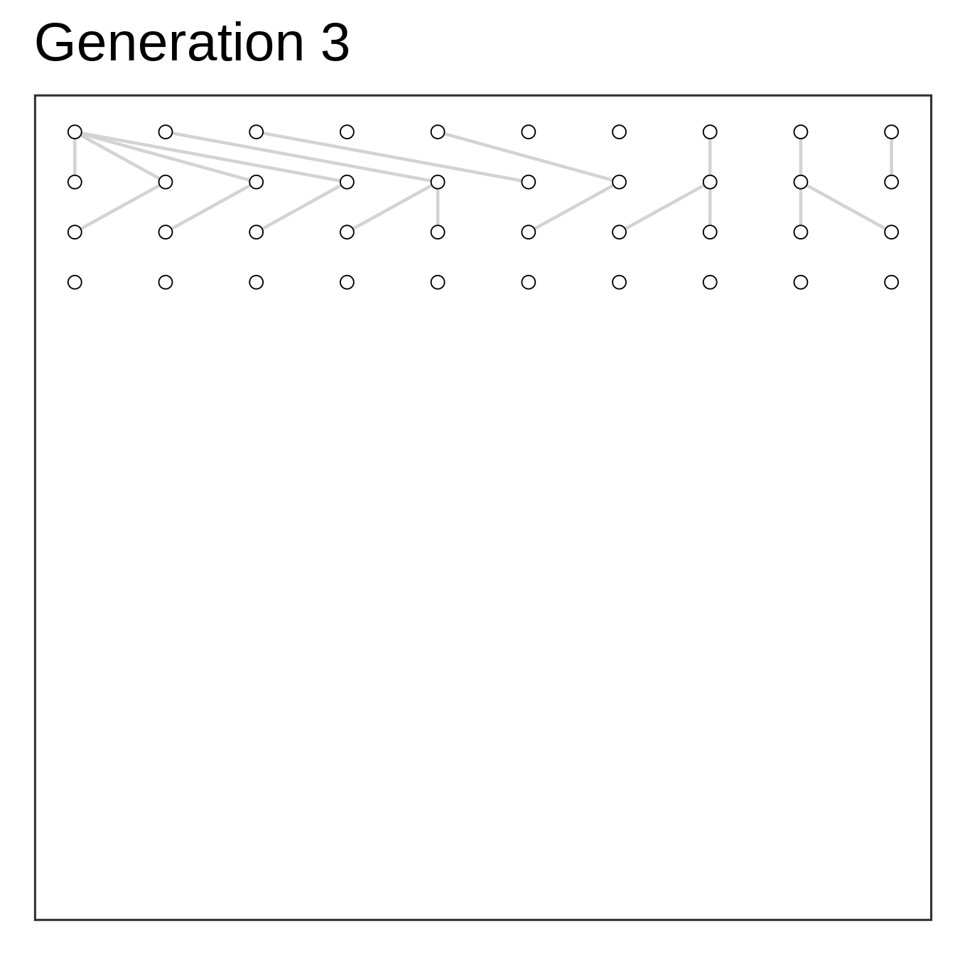
Wright-Fisher model


Observations
- most lineages are lost over time
- looking backwards in time genes eventually coalesce at a common ancestor
- looking backwards in time sampled genes can be described by a genealogy

Properties of Wright-Fisher sampling
The expected number of offspring is one

Poisson approximation for large N

P(v=k) \approx \frac{1}{k!}e^{-k}
Prob(pick same parent) = 1/2N

Time for two sequences to coalesce \sim 1/2N

Bibliography
Hein, J., Schierup, M. H., & Wiuf, C. (2005). Gene genealogies, variation and evolution: A primer in coalescent theory. Oxford University Press. https://books.google.se/books?id=CCmLNAEACAAJ
Hein, J., Schierup, M., & Wiuf, C. (2004). Gene genealogies, variation and evolution. A primer in coalescent theory. In Systematic Biology - SYST BIOL (Vol. 54).
Hermisson, J. (2017). Mathematical population genetics. https://www.mabs.at/fileadmin/user_upload/p_mabs/Lecture_Notes_2017