
Linkage disequilibrium
A first look at haplotype structure
Observations
- Particular combinations of alleles at different SNPs occur together
- Non-random assortment of alleles is called linkage disequilibrium (LD)
- Note: detecting LD does not ensure linkage or lack of equilibrium
- Unfortunate term: barrier to understanding (Slatkin, 2008)
Going forward: discuss how linkage generates LD and recombination breaks it down
Linkage generates haplotype structure


- Mutations 1, 2 on same branch \Rightarrow appear together
- Mutations 1, 5 on derived branches \Rightarrow usually appear together
Linkage disequilibrium in the absence of recombination

- we assume no homoplasy (back mutations)
- haplotypes consistent with single tree (without recombination) form perfect phylogeny
Recombination breaks association between loci
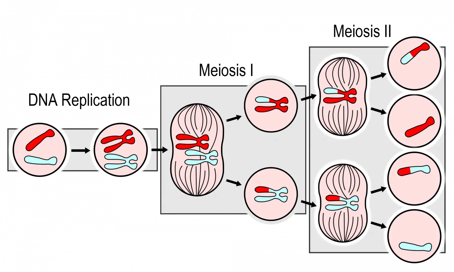
Miller (2020), Fig. 5.12.3
One (at least) crossover in meiosis I per chromosome! But: rates vary between loci (hotspots), sex chromosomes vs autosomes, and in some species, recombination only occurs in one sex (e.g., D.melanogaster).
Genetic distance and recombination rate

d - physical distance in bp
Definiton: genetic distance between two points is x centiMorgans(cM) if the average number of crossovers between points x/100 per meiosis
For short distances, genetic distance in cM \approx \mathrm{Pr}(\text{crossover})
Definition: recombination rate r relates genetic distance to base pair distance; commonly measured in cM/Mb
Example: in human average is 1.2 cM per Mb - the probability of crossover is a 1.2%
Recombination generates new combinations of alleles

Rules of thumb (human)
- For close SNPs (less than ~0.01-0.1 cM, or ~10-100Kb) linkage is stronger force than recombination
- At larger (>0.1cM) recombination is stronger
Measuring LD

Given only information about SNP allele frequencies p_A and p_B, what would guess be for p_{AB}?
If independent, then p_{AB} = p_Ap_B, else p_{AB} \neq p_Ap_B. We measure the deviation D
D = p_{AB} - p_Ap_B
and say that there is linkage equilibrium if D=0!
Alternative measures
Unfortunate property of D: its magnitude depends on allele frequencies!
\begin{align*} D^\prime = \frac{D}{D_\mathrm{max}} & = \frac{D}{\min(p_Ap_b,p_ap_B)}, \quad\mathrm{for\ }D>0\\ & = \frac{D}{\min(p_Ap_B,p_ap_b)}, \quad\mathrm{for\ }D<0 \end{align*}
|D^\prime| < 1 implies there must have been recombination
r^2 = \frac{D^2}{p_Ap_ap_Bp_b}
- r^2=1 perfect LD
- r^2 natural parameter for measuring contribution of LD to genetic associations
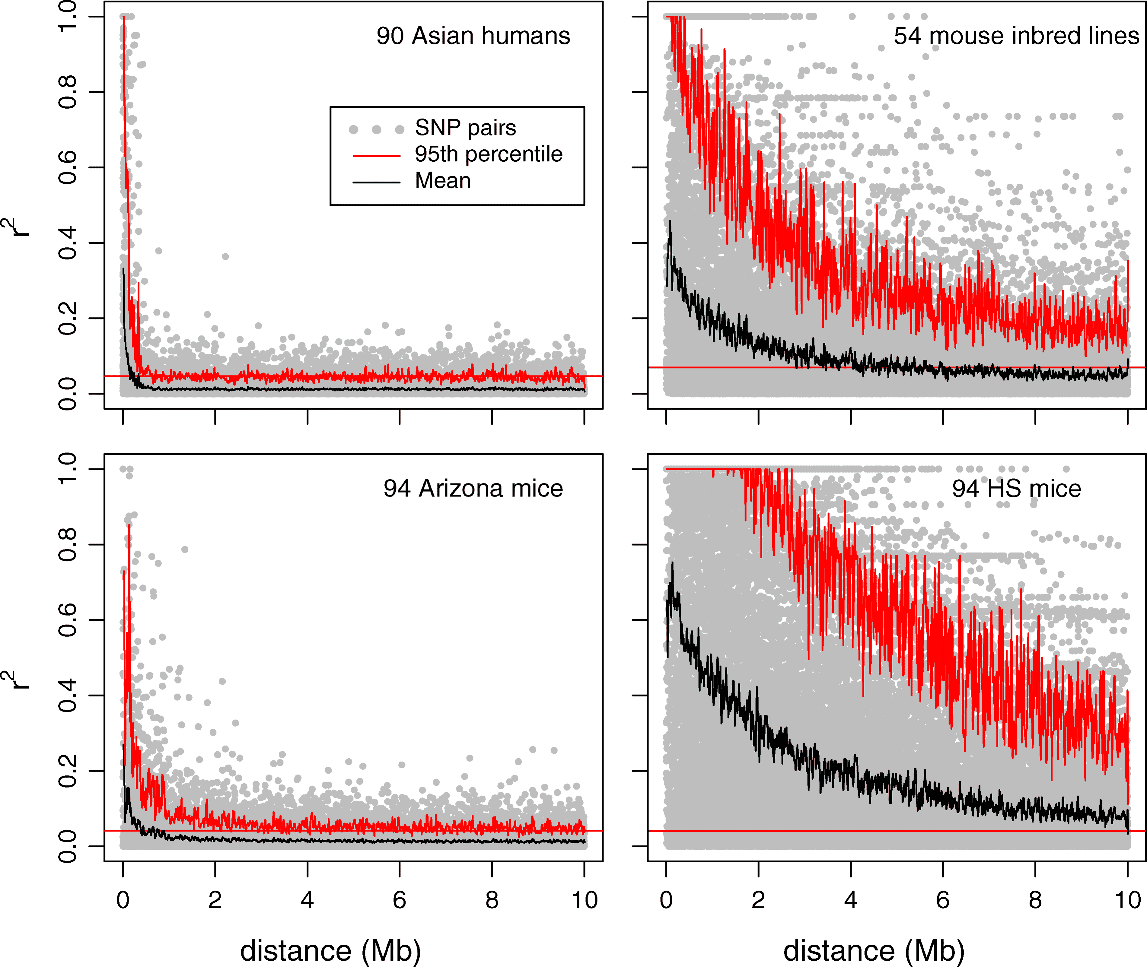
LD decay

Observation
Even for free recombination (r=0.5) LD decay takes time. Comparison: HWE which takes one generation.
Bibliography
Kreitman, M. (1983). Nucleotide polymorphism at the alcohol dehydrogenase locus of Drosophila melanogaster. Nature, 304(5925), 412. https://doi.org/10.1038/304412a0
Laurie, C. C., Nickerson, D. A., Anderson, A. D., Weir, B. S., Livingston, R. J., Dean, M. D., Smith, K. L., Schadt, E. E., & Nachman, M. W. (2007). Linkage Disequilibrium in Wild Mice. PLOS Genetics, 3(8), e144. https://doi.org/10.1371/journal.pgen.0030144
Miller, C. (2020). Human Biology. Thompson Rivers University.
Pritchard, J. K. (n.d.). An Owner’s Guide to the Human Genome. Retrieved August 18, 2025, from https://web.stanford.edu/group/pritchardlab/HGbook.html
Slatkin, M. (2008). Linkage disequilibrium — understanding the evolutionary past and mapping the medical future. Nature Reviews Genetics, 9(6), 477–485. https://doi.org/10.1038/nrg2361