Genetic diversity

Per Unneberg

What determines diversity levels?

The usual questions:

What evolutionary forces maintain genetic diversity in natural populations? How do diversity levels relate to census population sizes…? Do low levels of diversity limit adaptation to selective pressures?

Leffler et al. (2012)

After allozyme era, the study of genetic diversity was largely neglected due to lack of genome-wide data, but with advent of population genomics becoming a hot topic again.

Ellegren & Galtier (2016)

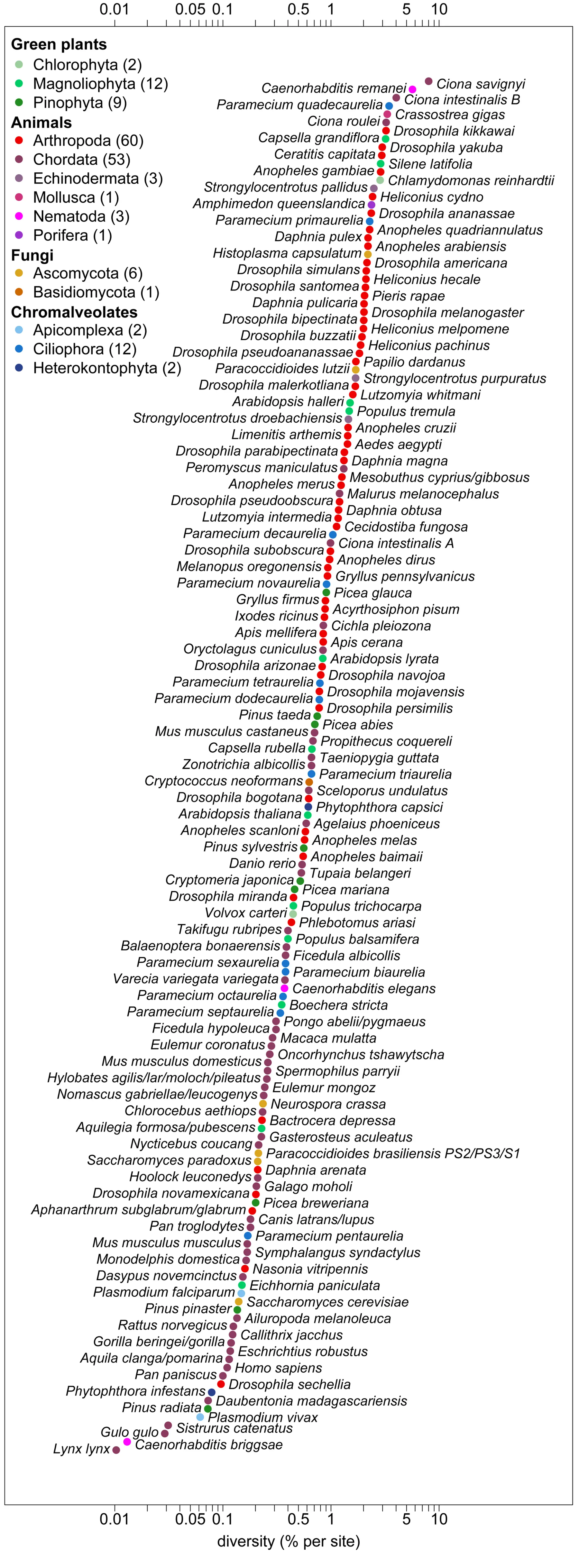
Lewontin’s paradox: genetic diversity range smaller than variation among species in population size

Riddle: why is genetic diversity range so narrow? Possibly there are lower and upper limits.

Lower limit: censoring effect, i.e., when diversity passes a lower limit, population is driven to extinction due to inability to adapt

Upper limit: functional/structural constraints, e.g., impaired chromosome pairing or reproductive incompatibilities

Linked selection, that is, variation-reducing selection. Larger populations have higher influx of new mutations, so if more draft, higher reduction in diversity. Would require strong frequent levels of selection; little support for this in literature.

Purifying selection. Nearly neutral model could explain narrow range.

(Ellegren & Galtier, 2016) Upper limit could in part be explained by linked selection (Corbett-Detig et al., 2015)

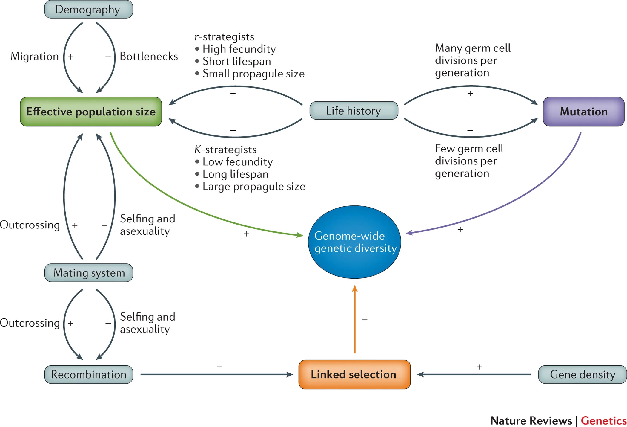
Factors that influence genetic diversity

Figure 1: Overview of determinants of genetic diversity (Ellegren & Galtier, 2016, Fig 2)

Genetic drift

Reduces diversity at loss \propto \frac{1}{N}

Selection

Adaptive selection decreases variation, more so if acting on new mutations compared to standing variation.

Balancing selection may increase variation.

Recombination

Low recombination rates lead to less “reshuffling” of variation and hence lower diversity.

Note: lower recombination lowers diversity presumably because more neutral variants linked to selected sites. There are intriguing differences between taxa (Leffler et al., 2012)

Ellegren & Galtier (2016) point out that with advent of population genomic data, we are at the brink of understanding Lewontin’s paradox, namely (Charlesworth & Jensen, 2022)

the observation that the range of levels of genetic diversity in natural populations appears to be far smaller than the extent of variation among species in population size

Why we measure patterns of genetic variation

Genetic variation patterns are informative of evolutionary and demographic processes. We often use summary statistics to describe the patterns, and to estimate parameters such as effective population size and mutation rate from genetic variation data (\theta = 4N_e\mu)

Often critical first step of analysis, such as

• exploratory study
• test of an evolutionary hypothesis
• training of machine-learning models

(Korunes & Samuk, 2021)

Genetic diversity in conservation biology

Figure 2: Kuderna et al. (2023), Fig 2

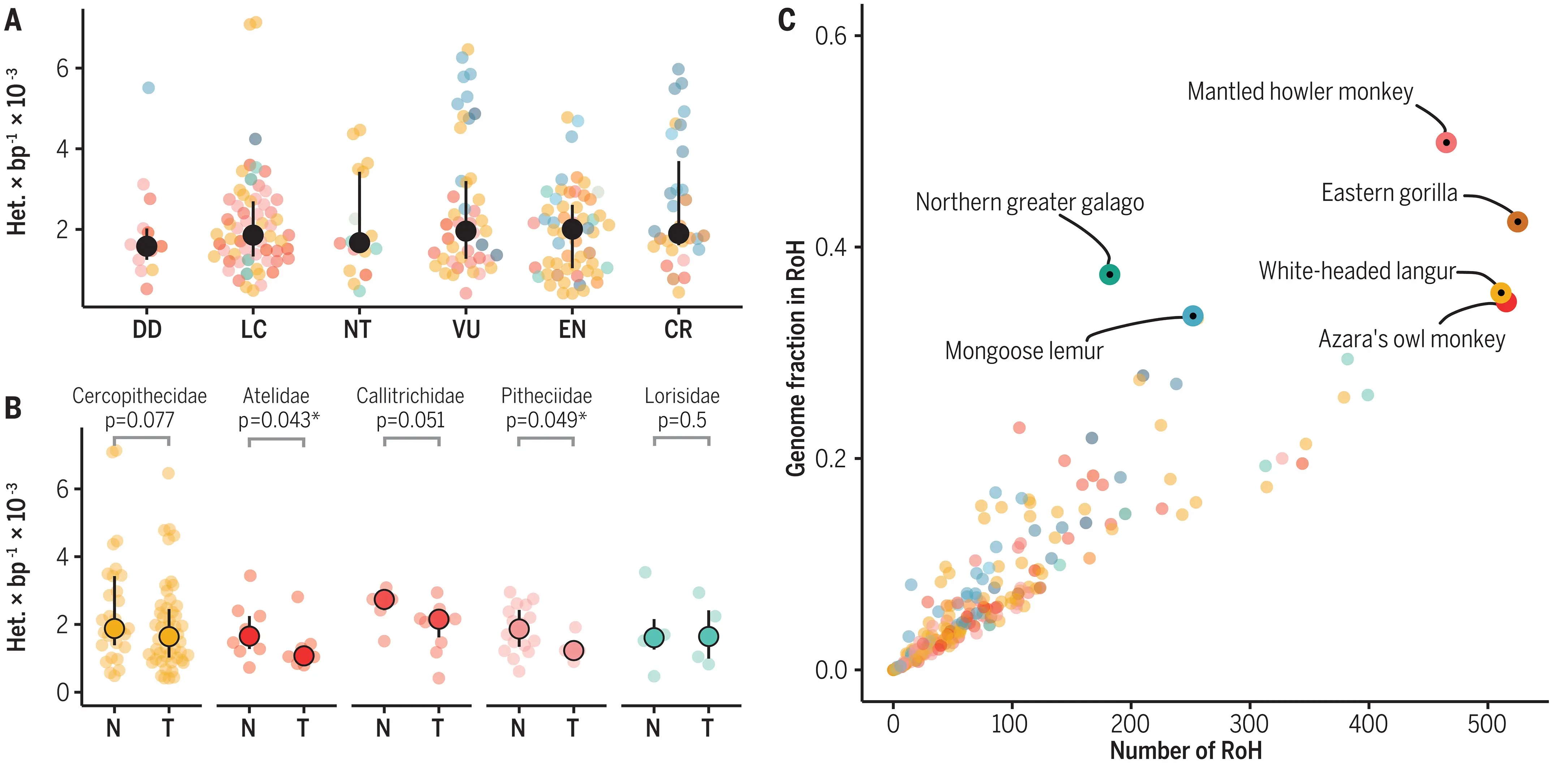
…no global relationship between numerically coded IUCN extinction risk categories and estimated heterozygosity…

Low genetic diversity symptom of past genetic drift inbreeding (higher levels of homozygosity), caused by low N_e

García-Dorado & Caballero (2021)

However: if population decline is rapid, may be too little time for inbreeding to occur \Rightarrow genetic diversity within species not necessarily aligned to extinction risk

Lewis (2023)

Take home (Lewis, 2023): genetic diversity within a species does not necessarily align with its extinction risk. Possible explanation: population decline has been so rapid that there hasn’t been time for inbreeding to occur. Other factors (e.g., habitat destruction) greater threat.

Caption:

Runs of homozygosity and impact of extinction risk on diversity (A) Relationship between IUCN extinction risk categories and heterozygosity. Solid black circles and bars denote median and IQR. (B) Partition into threatened (T: VU, EN, CR) and nonthreatened (N: LC, NT) categories for all families with more than one species in either partition. Significant differences (p < 0.05, one-sided rank-sum test) are marked with an asterisk. (C) Median number of tracts of homozygosity versus median proportion of the genome in runs of homozygosity per species. Species with a fraction over 1/3 are highlighted. Solid black dots within highlights denote threatened species (VU, EN, CR).

On Figure 2A:

We investigated whether genetic diversity estimates are correlated with extinction risk in primates, a subject of previous debate (17, 33, 34). Despite our broad sampling, we find no global relationship between numerically coded IUCN extinction risk categories and estimated heterozygosity [p > 0.05, phylogenetic generalized least squares (PGLS)] (Fig. 2A) (16).

Measuring genetic diversity

Nucleotide diversity

sample 0:   00100
sample 1:   00001
sample 2:   01010
sample 3:   10010

Diversity: for each site, count and sum differences between all (unique) pairs of samples, and divide by unique pairs. For n samples, there are n \choose 2 such pairs.

Example: for site 0, start comparing samples 0-1 (0 diffs), samples 0-2 (0), samples 0-3 (1), samples 1-2 (0) and so on. Call these differences k_{ij}. Then

\pi = \frac{\sum_{i<j}k_{ij}}{n \choose 2}

Tree plot with mutations and sequences

Watterson’s \theta_W

sample 0:   00100
sample 1:   00001
sample 2:   01010
sample 3:   10010

Alternative measure of diversity: simply count the number of segregating sites (S). However, must correct for the number of samples n as we expect that more samples \Rightarrow more sites

\theta_W = \frac{S}{a} = \frac{S}{\sum_{i=1}^{n-1}\frac{1}{i}}

Important: under neutrality, \theta = E(\pi) = E(\theta_W). Difference between two the basis for Tajima’s D that is a test for selection

Tree plot with mutations and sequences

Intuitive example to understand of Tajimas: balancing selection has long internal branches -> long haplotype. This will elevate pi since many samples will be different for many sites.

Calculating diversity measures - \pi and \theta_W

sample 0:   00100
sample 1:   00001
sample 2:   01010
sample 3:   10010

from trees import ts_small_mut as ts

# Calculate correction factor a for Watterson's
# theta: the larger the sample size, the more
# segregating sites we expect to see
a = sum([1/i for i in range(1, ts.num_samples)])

pi = ts.diversity()
thetaW = ts.num_sites / a / ts.sequence_length

print(f"Diversity:           {pi:.6f}",
      f"Watterson's theta:   {thetaW:.6f}",
      f"Sequence length:     {ts.sequence_length:.0f}",
      sep="\n")

Diversity:           0.000267
Watterson's theta:   0.000273
Sequence length:     10000

Tree plot with mutations and sequences

Divergence - dXY

Sample 0:   00100
Sample 1:   00001

Sample 2:   01010
Sample 3:   10010

Divergence: for each site, count and sum differences between all pairs of samples between two populations

Example: for site 0, compare samples 0-2 (0 diffs), samples 0-3 (1 diff), samples 1-2 (0 diffs), samples 1-3 (1 diff), and so on. Call differences k_ij, let n_X, n_Y be sample size in populations X, Y. Then

d_{XY} = \frac{1}{n_Xn_Y}\sum_{i=1}^{n_X}\sum_{i=1}^{n_Y}k_{ij}

Tree plot with mutations and sequences

Divergence - dXY

Sample 0:   00100
Sample 1:   00001

Sample 2:   01010
Sample 3:   10010

from trees import ts_small_mut as ts

sample_sets = [[0, 1], [2, 3]]

dxy = ts.divergence(sample_sets=sample_sets)

print(f"Divergence:   {dxy:.6f}")

Divergence:   0.000300

Tree plot with mutations and sequences

F_ST (later) and related statistics are strongly affected by within-subpopulation genetic variance. Nei (1973) proposed dXY as an alternative that does not depend on the levels of diversity within subpopulations.

Differentiation - AFD (allele frequency difference)

Sample 0:   00100
Sample 1:   00001

Sample 2:   01010
Sample 3:   10010

Allele Frequency Difference (AFD) proposed as intuitive alternative to F_{\mathrm{ST}}. For each site, count the difference in allele frequency between two populations.

Example: site 0, frequency in blue is 0, in black 1/2, so difference=1/2, site 1, frequency in blue 0, in black 1/2, and so on

AFD = \frac{1}{2}\sum_{i=1}^n| (f_{i1} - f_{i2})|

where n is the number of different alleles (n=2 for biallelic SNPs), f_{ij} is the frequency of allele i in population j

Berner (2019)

Tree plot with mutations and sequences

AFD proposed as a more intuitive and easier to understand statistic than Fst

Differentiation - F_{\mathrm{ST}}

Sample 0:   00100
Sample 1:   00001

Sample 2:   01010
Sample 3:   10010

F_{\mathrm{ST}} is another measure of differention among subpopulations (Wright, 1931). It ranges between 0 and 1 and has the interpretation 0: no differentiation, 1: complete fixation of alternate alleles in subpopulations

Example: site 3 has F_{\mathrm{ST}}=1 as it is fixed in black, not present in blue

There are many ways to express and calculate F_{\mathrm{ST}}. Example:

F_{\mathrm{ST}} = \frac{h_{\mathrm{T}} - h_{\mathrm{S}}}{h_{\mathrm{T}}}

where h_{\mathrm{T}} is the expected heterozygosity in the total population, h_{\mathrm{S}} the average of expected heterozygosities across subpopulations. For site 3, h_{\mathrm{S}}=0, h_{\mathrm{T}}=2/3.

Caveats: strongly influenced by within subpopulation levels of variation. Therefore considered relative measure (cf d_{\mathrm{XY}}, which is an absolute measure).

Tree plot with mutations and sequences

Wright’s fst measures differentiation among subpopulations. Interpretation: 0 no differentiation, 1 complete fixation of alternate alleles. Has therefore become a popular statistic for quantifying differentiation from molecular data.

Differentiation - F_{\mathrm{ST}}

Sample 0:   00100
Sample 1:   00001

Sample 2:   01010
Sample 3:   10010

from trees import ts_small_mut as ts

sample_sets = [[0, 1], [2, 3]]
win = [0] + [int(x.position)+1 for x in ts.sites()]
_ = win.pop()
win = win + [ts.sequence_length]

fst = ts.Fst(sample_sets=sample_sets)
fst_sites = ts.Fst(sample_sets=sample_sets,
                   windows=win)

print(f"Site id:       {list(range(5))}",
      f"Fst per site:  {fst_sites}",
      f"Overall Fst:   {fst:.6f}",
      sep="\n")

Site id:       [0, 1, 2, 3, 4]
Fst per site:  [0. 0. 0. 1. 0.]
Overall Fst:   0.200000

Tree plot with mutations and sequences

Many programs treat missing data as invariant

Korunes & Samuk (2021), Fig 1

Diversity:

\pi = \frac{\sum_{i<j}k_{ij}}{n \choose 2}

Divergence:

d_{XY} = \frac{1}{n_Xn_Y}\sum_{i=1}^{n_X}\sum_{j=1}^{n_Y}k_{ij}

Here, n is the number of samples, k_{ij} tally of allelic differences between two haplotypes within (\pi) a population or between (d_{XY}) populations

Paper caption:

The logic and input/ouput of pixy demonstrated with a simple haploid example. (a) Comparison of two methods for computing π (or dXY) in the face of missing data. These methods follow the first expression of Equation 1 but differ in how they calculate the numerator and denominator. In Case 1, all missing data is assumed to be present but invariant. This results in a deflated estimate of π. In Case 2, missing data are simply omitted from the calculation, both in terms of the number of sites (the final denominator) and the component denominators for each site (the n choose two terms). This results in an unbiased estimate of π. (b) The adjusted π method (Case 2) as implemented for VCFs in pixy. The example VCF (input) contains the same four haplotypes as (a). Invariant sites are represented as sites with no ALT allele, and greyed-out sites are those that failed to pass a genotype filter requiring a minimum number of reads covering the genotype (Depth ≥ 10 in this case)

Missing data may bias diversity measures downwards

Korunes & Samuk (2021), Fig 4

Real data: strong tendency of commonly adopted tools to underestimate pi, dxy (even for 30X data sets)

Caption:

Comparisons of estimates of π from whole genome data derived from 18 Anopheles gambiae individuals from the Ag1000G Burkina Faso (BFS) population. Each panel (a–d) depicts the estimates of π for the X chromosome performed using pixy (y-axis) and four other methods (x-axis, a–d). Points are coloured according to the proportion of missing data (of any type) calculated by pixy. The 1:1 line is shown in red

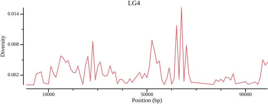
Nucleotide diversity landscapes

vcftools --gzvcf vcf/allsites.vcf.gz --window-pi 1000 --out results/out
csvtk plot line --tabs results/out.windowed.pi -x BIN_START -y PI \
   --point-size 0.01 --xlab "Position (bp)" \
   --ylab "Diversity" --title LG4 --width 9.0 --height 3.5 \
   > results/out.windowed.pi.png

Window-based plot is seque into genome scans

On genome scans

Genetic basis of adaptation and genome scans

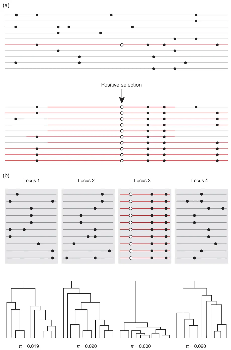
Fundamental questions:

• How many genes are involved in the evolution of adaptive traits?
• What is the distribution of phenotypic effects among successive allelic substitutions?
• Is adaptation typically based on standing variation or new mutations?
• What is the relative importance of additive vs. nonadditive effects on adaptive trait variation?
• And what is the relative importance of structural vs. regulatory changes in phenotypic evolution?

Storz (2005), Fig 1

Storz (2005) lays out genomic scans as an alternative approach to GWAS and QTL mapping for finding genetic determinants of adaptation. The reason is GWAS/QTL requires a phenotype whereas genome scans are data-driven.

Caption (fig 1):

Fig. 1 (a) Effects of genetic hitch-hiking along a recombining chromosome. Hori- zontal lines depict a population sample of homologous chromosomes, and filled symbols depict neutral mutations. In this example an advantageous mutation (open symbol) arises and is rapidly driven to fixation by positive selection. Although the mutation is recombined against new genetic backgrounds during the course of the selective sweep, a sizable fraction of the ancestral haplotype (shown in red) also becomes fixed. Consequently, neutral variants that were initially linked to the advantageous mutation undergo a dramatic increase in frequency as a result of hitchhiking. (b) In this example, locus 3 has been rendered monomorphic by a selective sweep. Sampled gene copies (denoted by tips of the gene tree) share a very recent common ancestor, and π = 0 (where π = nucleotide diversity; Nei & Li 1979). comparison, unlinked, neutrally evolving regions of the genome (loci 1, 2, and 4) are characterized by deeper genealogies, and higher levels of nucleotide diversity (π = 0.019–0.020). Note that the gene trees depict the true genealogies of the samples, not the genealogies inferred from observed variation.

Example

vcftools --gzvcf vcf/allsites.vcf.gz --weir-fst-pop PUN-Y.txt \
   --weir-fst-pop PUN-R.txt \
   --fst-window-size 1000 \
   --out results/out
csvtk plot line --tabs results/out.windowed.weir.fst \
   -x BIN_START -y MEAN_FST \
   --point-size 2 --xlab "Position (bp)" \
   --ylab "Fst" --title "LG4: PUN-Y vs PUN-R" \
   --width 9.0 --height 3.5 --scatter \
   > results/out.windowed.weir.fst.mean.png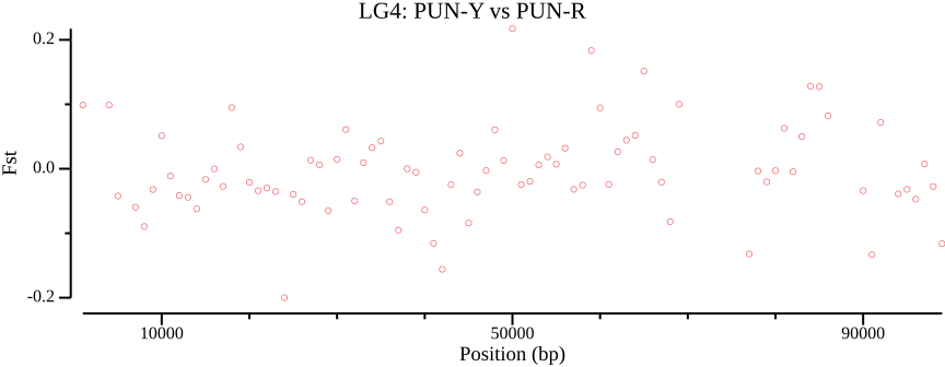

Z-scores can help identifying outliers

data <- read.table("results/out.windowed.weir.fst", header = TRUE)
x <- data$MEAN_FST
z <- (x - mean(x))/sd(x)
plot(x = data$BIN_START, y = z, xlab = "Position (bp)")

Raw data can be converted to Z-scores to highlight outliers. A Z-score is a measure of how far a data point is from the mean in terms of the number of standard deviations:

Z = \frac{X - \mu}{\sigma}

Threshold of a couple of standard deviations common.

LD decay and choice of window size

Properties of genetic variation and inferred demographic history in sampled A. millepora. Fuller et al. (2020), Figure 2. Upper left plot illustrates LD as a function of physical distance. Here, choosing a window size 20-30kb would ensure that most windows are independent.

Annotations

csvtk filter2 --tabs gff/annotation.gff --filter ' $3 == "CDS" ' |\
 csvtk mutate2 --tabs -H -e '$4 - 12000000' -w 0 |\
 csvtk mutate2 --tabs -H -e '$5 - 12000000' -w 0 |\
 csvtk cut --tabs --fields 1,10,11 | bedtools sort | bedtools merge \
    > bed/CDS.bed 2>/dev/null
head -n 3 bed/CDS.bed

LG4 12032   12121
LG4 12214   12658
LG4 12774   12830

pixy --vcf vcf/allsites.vcf.gz --stats pi \
 --populations populations.txt --output_prefix cds \
 --output_folder results --bed_file bed/CDS.bed
pixy --vcf vcf/allsites.vcf.gz --stats pi \
 --populations populations.txt --window_size 1000 \
 --output_prefix all --output_folder results

csvtk summary --tabs -i -g pop \
   -f avg_pi:mean results/cds_pi.txt -w 5

pop avg_pi:mean
PUN-R   0.00247
PUN-Y   0.00462

csvtk summary --tabs -i -g pop \
   -f avg_pi:mean results/all_pi.txt -w 5

pop avg_pi:mean
PUN-R   0.00893
PUN-Y   0.00805

Genome diversity and differentiation landscapes

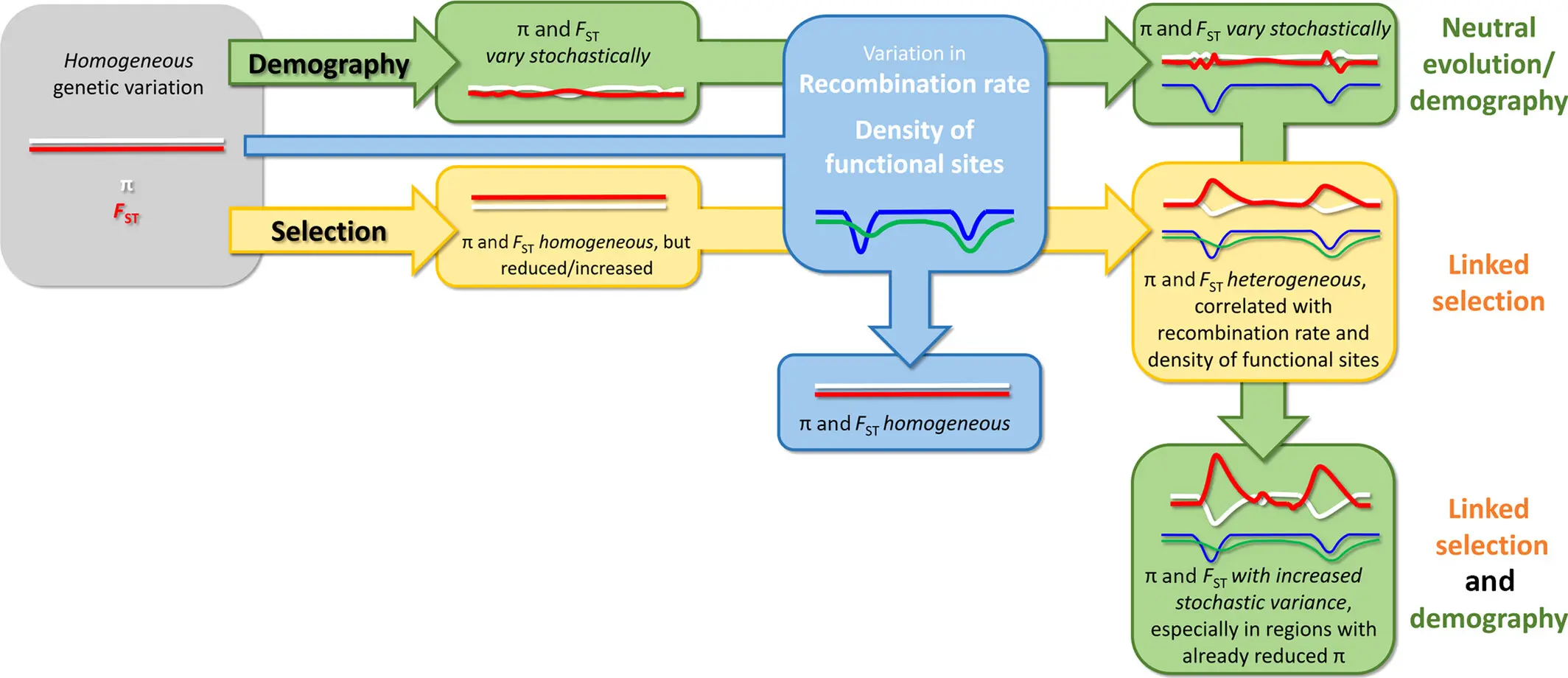
Dissecting differentiation landscapes

Figure 3: Burri (2017) Fig. 1

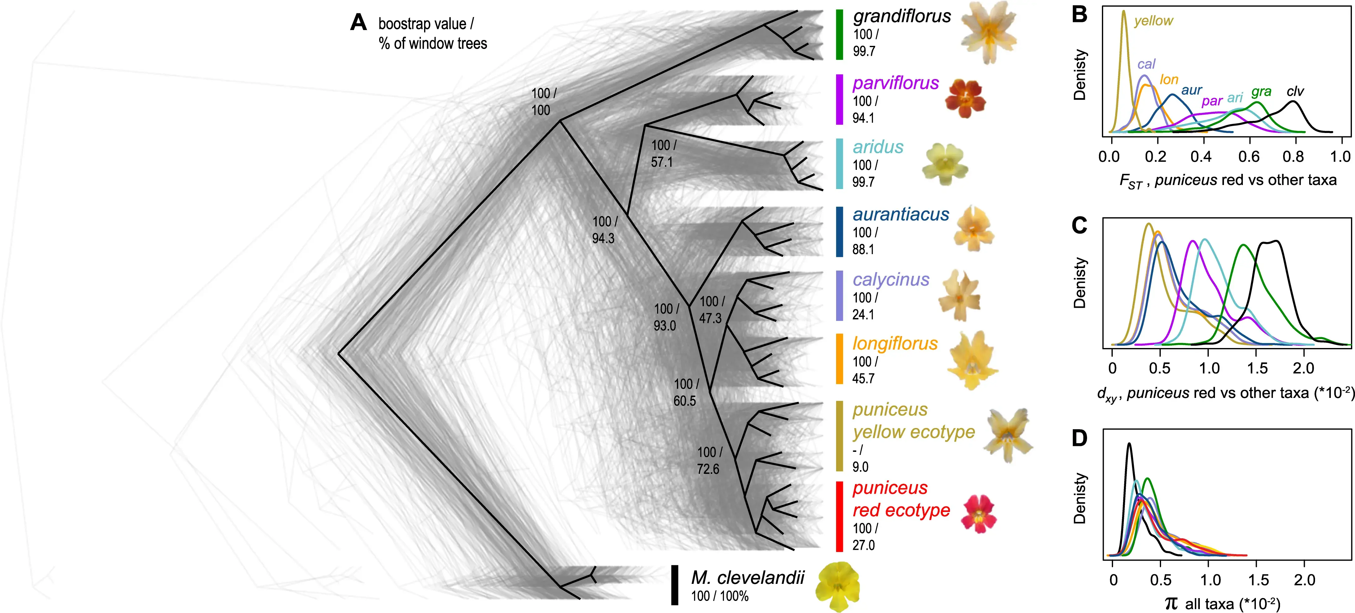
Monkeyflower genomic landscape

Figure 4: Stankowski et al. (2019) Fig. 1

Exercise

Bibliography

Berner, D. (2019). Allele Frequency Difference AFD to FST for Quantifying Genetic Population Differentiation. Genes, 10(4), 308. https://doi.org/10.3390/genes10040308

Burri, R. (2017). Dissecting differentiation landscapes: A linked selection’s perspective. Journal of Evolutionary Biology, 30(8), 1501–1505. https://doi.org/10.1111/jeb.13108

Charlesworth, B., & Jensen, J. D. (2022). How Can We Resolve Lewontin’s Paradox? Genome Biology and Evolution, 14(7), evac096. https://doi.org/10.1093/gbe/evac096

Corbett-Detig, R. B., Hartl, D. L., & Sackton, T. B. (2015). Natural Selection Constrains Neutral Diversity across A Wide Range of Species. PLOS Biology, 13(4), e1002112. https://doi.org/10.1371/journal.pbio.1002112

Ellegren, H., & Galtier, N. (2016). Determinants of genetic diversity. Nature Reviews Genetics, 17(7), 422–433. https://doi.org/10.1038/nrg.2016.58

Fuller, Z. L., Mocellin, V. J. L., Morris, L. A., Cantin, N., Shepherd, J., Sarre, L., Peng, J., Liao, Y., Pickrell, J., Andolfatto, P., Matz, M., Bay, L. K., & Przeworski, M. (2020). Population genetics of the coral Acropora millepora: Toward genomic prediction of bleaching. Science, 369(6501), eaba4674. https://doi.org/10.1126/science.aba4674

García-Dorado, A., & Caballero, A. (2021). Neutral genetic diversity as a useful tool for conservation biology. Conservation Genetics, 22(4), 541–545. https://doi.org/10.1007/s10592-021-01384-9

Korunes, K. L., & Samuk, K. (2021). Pixy: Unbiased estimation of nucleotide diversity and divergence in the presence of missing data. Molecular Ecology Resources, 21(4), 1359–1368. https://doi.org/10.1111/1755-0998.13326

Kuderna, L. F. K., Gao, H., Janiak, M. C., Kuhlwilm, M., Orkin, J. D., Bataillon, T., Manu, S., Valenzuela, A., Bergman, J., Rousselle, M., Silva, F. E., Agueda, L., Blanc, J., Gut, M., de Vries, D., Goodhead, I., Harris, R. A., Raveendran, M., Jensen, A., … Marques Bonet, T. (2023). A global catalog of whole-genome diversity from 233 primate species. Science, 380(6648), 906–913. https://doi.org/10.1126/science.abn7829

Leffler, E. M., Bullaughey, K., Matute, D. R., Meyer, W. K., Ségurel, L., Venkat, A., Andolfatto, P., & Przeworski, M. (2012). Revisiting an Old Riddle: What Determines Genetic Diversity Levels within Species? PLOS Biology, 10(9), e1001388. https://doi.org/10.1371/journal.pbio.1001388

Lewis, D. (2023). Biggest ever study of primate genomes has surprises for humanity. Nature. https://doi.org/10.1038/d41586-023-01776-6

Nei, M. (1973). Analysis of Gene Diversity in Subdivided Populations. Proceedings of the National Academy of Sciences, 70(12), 3321–3323. https://doi.org/10.1073/pnas.70.12.3321

Stankowski, S., Chase, M. A., Fuiten, A. M., Rodrigues, M. F., Ralph, P. L., & Streisfeld, M. A. (2019). Widespread selection and gene flow shape the genomic landscape during a radiation of monkeyflowers. PLOS Biology, 17(7), e3000391. https://doi.org/10.1371/journal.pbio.3000391

Storz, J. F. (2005). INVITED REVIEW: Using genome scans of DNA polymorphism to infer adaptive population divergence. Molecular Ecology, 14(3), 671–688. https://doi.org/10.1111/j.1365-294X.2005.02437.x

Wright, S. (1931). Evolution in Mendelian Populations. Genetics, 16(2), 97–159. https://www.ncbi.nlm.nih.gov/pmc/articles/PMC1201091/