24 Exercises: Survival analysis

library(tidyverse)
library(gtsummary) # for tables
library(survival) #survival functions
library(survminer) #for ggsurvplot
library(cmprsk) #competing risks

24.1 Kaplan-Meier curves and log-rank test

Exercise 24.1 (Brain cancer survival) The dataset data_cancer_brain.rds contains survival data for patients with primary brain tumors.

Load the data and inspect the variables. The variable status indicates whether the event was observed (1) or the observation was censored (0).

data_brain <- readRDS("data/data_cancer_brain.rds")
tbl_summary(data_brain)

Table 24.1: Summary of the brain data set.

Characteristic	N = 88¹
sex
Female	45 (51%)
Male	43 (49%)
diagnosis
Meningioma	42 (48%)
LG glioma	9 (10%)
HG glioma	22 (25%)
Other	14 (16%)
Unknown	1
loc
Infratentorial	19 (22%)
Supratentorial	69 (78%)
ki
40	1 (1.1%)
60	5 (5.7%)
70	14 (16%)
80	36 (41%)
90	27 (31%)
100	5 (5.7%)
gtv	7 (3, 12)
stereo
SRS	23 (26%)
SRT	65 (74%)
status	35 (40%)
time	24 (10, 42)
¹ n (%); Median (Q1, Q3)

Plot a Kaplan-Meier curve for the full dataset.
Plot Kaplan-Meier curves stratified by sex.
Based on the plot, do men and women appear to have similar survival patterns?
Use a log-rank test to formally compare the survival curves.

Solution

Kaplan-Meier curve for all patients:

fit.surv <- survfit(Surv(time, status) ~ 1, data = data_brain)
plot(fit.surv, xlab = "Months", ylab = "Estimated Probability of Survival")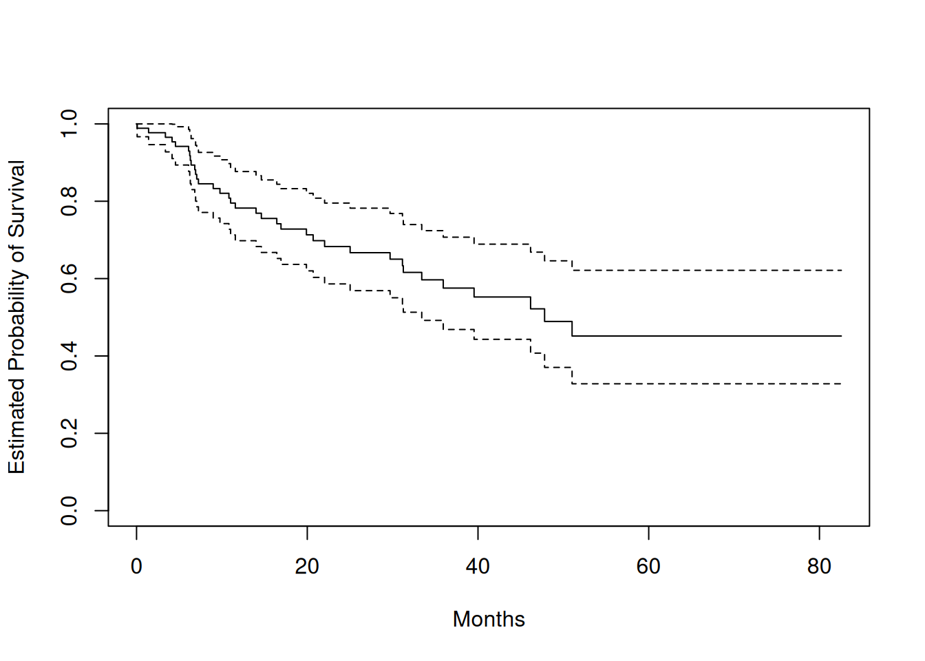


##or plot using ggsurvplot
ggsurvplot(fit.surv)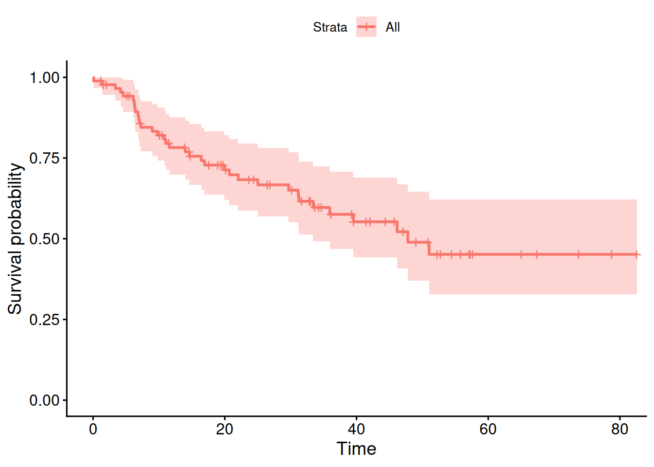

Kaplan-Meier curves by sex:

fit.sex <- survfit(Surv(time, status) ~ sex, data = data_brain)
ggsurvplot(fit.sex)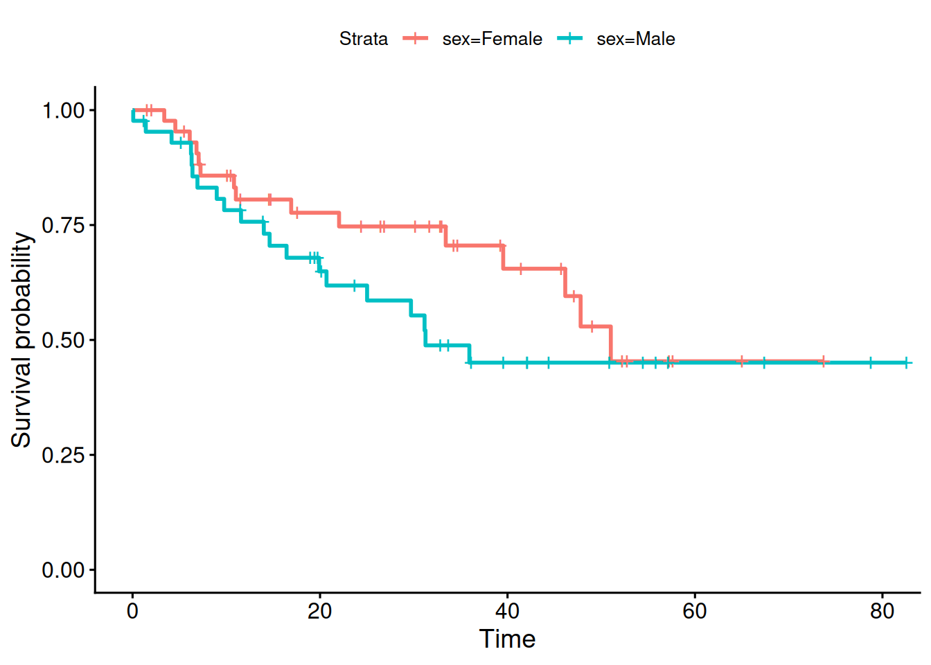

The curves can be compared visually. If they are clearly separated, this suggests possible differences in survival, although a formal statistical test is needed.

Select an appropriate significance level and perform the log-rank test. Is there a difference in survival time between males and females?

logrank_test <- survdiff(Surv(time, status) ~ sex, data = data_brain)
logrank_test
## Call:
## survdiff(formula = Surv(time, status) ~ sex, data = data_brain)
## 
##             N Observed Expected (O-E)^2/E (O-E)^2/V
## sex=Female 45       15     18.5     0.676      1.44
## sex=Male   43       20     16.5     0.761      1.44
## 
##  Chisq= 1.4  on 1 degrees of freedom, p= 0.2
##Compute p-value
pchisq(logrank_test$chisq, df = length(logrank_test$n) - 1, lower.tail = FALSE)
## [1] 0.2300592

## The logrank p-value can be printed easily in the ggsurvplot
ggsurvplot(fit.sex, pval=TRUE)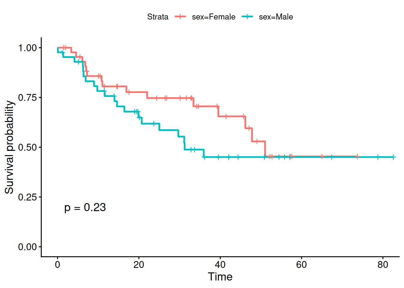

24.2 Cox regression

Exercise 24.2 (Cox proportional hazards model) Continue with the brain cancer dataset.

Fit a Cox proportional hazards model with sex as predictor.
Interpret the hazard ratio for sex.
Test the proportional hazards assumption.
Fit a Cox model with several predictors: sex, diagnosis, loc, ki, gtv, and stereo.
Which predictors appear to be important?

Solution

Cox model with sex only:

fit.cox <- coxph(Surv(time, status) ~ sex, data = data_brain)
summary(fit.cox)
## Call:
## coxph(formula = Surv(time, status) ~ sex, data = data_brain)
## 
##   n= 88, number of events= 35 
## 
##           coef exp(coef) se(coef)     z Pr(>|z|)
## sexMale 0.4077    1.5033   0.3420 1.192    0.233
## 
##         exp(coef) exp(-coef) lower .95 upper .95
## sexMale     1.503     0.6652     0.769     2.939
## 
## Concordance= 0.565  (se = 0.045 )
## Likelihood ratio test= 1.44  on 1 df,   p=0.2
## Wald test            = 1.42  on 1 df,   p=0.2
## Score (logrank) test = 1.44  on 1 df,   p=0.2

The hazard ratio for sex is obtained as exp(coef). It compares the hazard of the event between the sex groups. If the HR is above 1, the hazard is higher in the coded comparison group; if it is below 1, the hazard is lower.
Test the proportional hazards assumption:

ph_test <- cox.zph(fit.cox)
print(ph_test)
##        chisq df    p
## sex    0.588  1 0.44
## GLOBAL 0.588  1 0.44
plot(ph_test)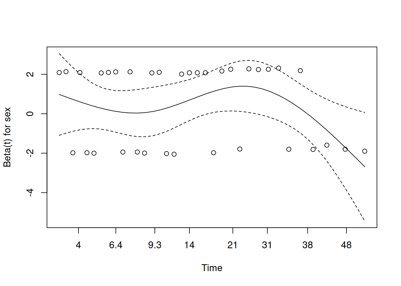

If the p-value is small, this suggests evidence against the proportional hazards assumption.

The proportional hazards assumption appears reasonable, we may proceed with this Cox model.

Cox model with multiple predictors:

fit.cox_multi <- coxph(Surv(time, status) ~ sex + diagnosis + loc + ki + gtv + stereo, data = data_brain)
summary(fit.cox_multi)
## Call:
## coxph(formula = Surv(time, status) ~ sex + diagnosis + loc + 
##     ki + gtv + stereo, data = data_brain)
## 
##   n= 87, number of events= 35 
##    (1 observation deleted due to missingness)
## 
##                        coef exp(coef) se(coef)      z Pr(>|z|)    
## sexMale             0.18375   1.20171  0.36036  0.510  0.61012    
## diagnosisLG glioma  0.91502   2.49683  0.63816  1.434  0.15161    
## diagnosisHG glioma  2.15457   8.62414  0.45052  4.782 1.73e-06 ***
## diagnosisOther      0.88570   2.42467  0.65787  1.346  0.17821    
## locSupratentorial   0.44119   1.55456  0.70367  0.627  0.53066    
## ki                 -0.05496   0.94653  0.01831 -3.001  0.00269 ** 
## gtv                 0.03429   1.03489  0.02233  1.536  0.12466    
## stereoSRT           0.17778   1.19456  0.60158  0.296  0.76760    
## ---
## Signif. codes:  0 '***' 0.001 '**' 0.01 '*' 0.05 '.' 0.1 ' ' 1
## 
##                    exp(coef) exp(-coef) lower .95 upper .95
## sexMale               1.2017     0.8321    0.5930    2.4352
## diagnosisLG glioma    2.4968     0.4005    0.7148    8.7215
## diagnosisHG glioma    8.6241     0.1160    3.5664   20.8546
## diagnosisOther        2.4247     0.4124    0.6678    8.8031
## locSupratentorial     1.5546     0.6433    0.3914    6.1741
## ki                    0.9465     1.0565    0.9132    0.9811
## gtv                   1.0349     0.9663    0.9906    1.0812
## stereoSRT             1.1946     0.8371    0.3674    3.8839
## 
## Concordance= 0.794  (se = 0.04 )
## Likelihood ratio test= 41.37  on 8 df,   p=2e-06
## Wald test            = 38.7  on 8 df,   p=6e-06
## Score (logrank) test = 46.59  on 8 df,   p=2e-07

The diagnosisHG glioma and ki seems important, based on their low p-values.

24.3 Adjusted survival curves from a Cox model

Exercise 24.3 (Predicted survival curves by diagnosis) Continue with the Cox model with many predictors from Exercise 24.2.

We now want to compare the predicted survival curves for the different diagnosis groups while keeping the other predictors fixed.

Construct a small data frame with one row for each diagnosis category.

Set sex = "Female", loc = "Supratentorial", stereo = "SRT", and use the sample means of ki and gtv.

modeldata <- data.frame(
  diagnosis = levels(data_brain$diagnosis),
  sex = rep("Female", length(levels(data_brain$diagnosis))),
  loc = rep("Supratentorial", length(levels(data_brain$diagnosis))),
  ki = rep(mean(data_brain$ki), length(levels(data_brain$diagnosis))),
  gtv = rep(mean(data_brain$gtv), length(levels(data_brain$diagnosis))),
  stereo = rep("SRT", length(levels(data_brain$diagnosis)))
)
modeldata
##    diagnosis    sex            loc       ki      gtv stereo
## 1 Meningioma Female Supratentorial 81.02273 8.660795    SRT
## 2  LG glioma Female Supratentorial 81.02273 8.660795    SRT
## 3  HG glioma Female Supratentorial 81.02273 8.660795    SRT
## 4      Other Female Supratentorial 81.02273 8.660795    SRT

Use survfit() and plot the predicted survival curves for the diagnosis groups using e.g. ggsurvplot.
Which diagnosis group appears to have the best predicted survival under the chosen covariate values?

Solution

Predicted survival curves:

survplots <- survfit(fit.cox_multi, newdata = modeldata)
ggsurvplot(
  survplots,
  data = modeldata,
  legend.labs = modeldata$diagnosis,
  legend.title = "Diagnosis",
  xlab = "Months",
  conf.int = FALSE
)

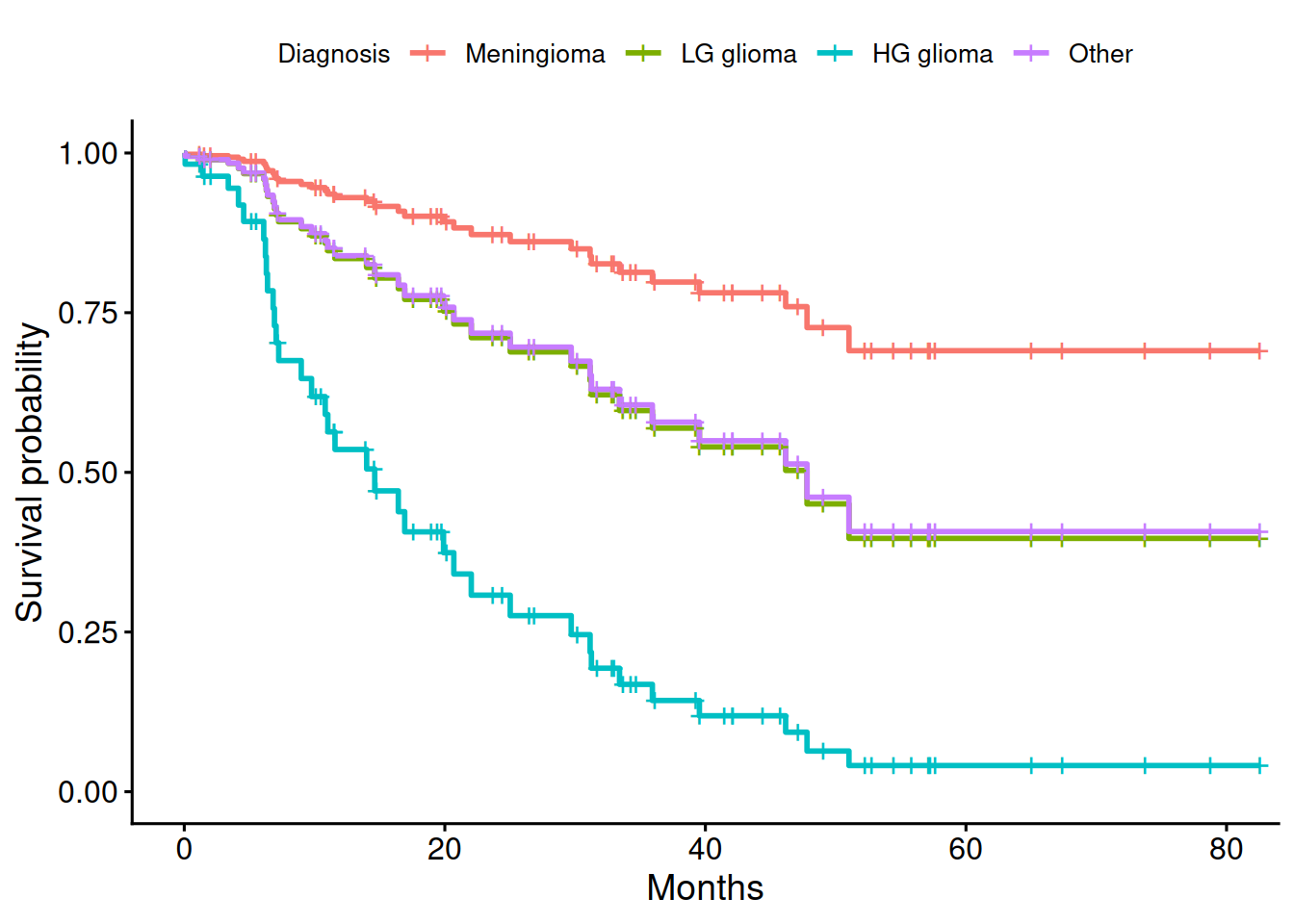
The diagnosis group Meningioma with the highest curve has the best predicted survival under the chosen covariate values.

24.4 Time-varying predictors

adpoted from https://www.bookdown.org/rwnahhas/RMPH/

A dataset with time-varying predictors will have multiple rows per individual, with different rows having different values for the time-varying predictors, reflecting how they change over time. Additionally, rather than having a single event time variable, each row will have two time variables indicating the beginning and end of the time interval represented by that row of data.

Use the opiod dataset: data/data-opioid.rds.

data_opioid <- readRDS("data/data-opioid.rds")

data_opioid %>% 
  filter(RANDID == 10) %>%
  select(RANDID, wave, START, STOP, heroin, age_at_init, sex, dep_lifetime)
##   RANDID wave START STOP heroin age_at_init  sex dep_lifetime
## 1     10    1  3.78 4.26      0          19 Male            0
## 2     10    2  4.26 4.78      0          19 Male            1
## 3     10    3  4.78 5.29      0          19 Male            1
## 4     10    4  5.29 5.84      0          19 Male            1
## 5     10    5  5.84 6.27      0          19 Male            1
## 6     10    6  6.27 6.79      1          19 Male            1

Here, we see a preview of the data_opioid dataset containing longitudinal information for 362 individuals, who at baseline had used non-prescribed pharmaceutical opioids (NPPO, “pain pills”), but were not dependent on NPPOs and had never used heroin.

Each row contains the time variables START and STOP which define the time interval (years from initiation of NPPO use) associated with that row.
Time-invariant variables in the dataset are constant over all rows for the same individual, while time-varying variables can change between rows.
Each (START, STOP] interval defines a period of time during which no variables changed.
Two time-varying variables in the dataset are heroin use (heroin) (the event indicator variable) and lifetime opioid dependence (dep_lifetime)
For instance, for this particular individual, male, started using NPPOs at age 19 (time invariant variables). He did not meet the criteria for lifetime opioid dependence at baseline (wave = 0), but did at the next interview (wave = 1) and he first reported using heroin at his 6th interview.

To model the heroin usage using both time-invariant and time-varying predictors, we can use the coxph function:

cox.timevar <- coxph(Surv(START, STOP, heroin) ~
                     age_at_init + sex + dep_lifetime, cluster = RANDID,
                   data = data_opioid)

summary(cox.timevar)
## Call:
## coxph(formula = Surv(START, STOP, heroin) ~ age_at_init + sex + 
##     dep_lifetime, data = data_opioid, cluster = RANDID)
## 
##   n= 1853, number of events= 27 
## 
##                 coef exp(coef) se(coef) robust se      z Pr(>|z|)   
## age_at_init  -0.3932    0.6749   0.1350    0.1247 -3.153  0.00161 **
## sexMale       0.1515    1.1635   0.3925    0.3831  0.395  0.69254   
## dep_lifetime  1.0580    2.8807   0.3991    0.3850  2.748  0.00600 **
## ---
## Signif. codes:  0 '***' 0.001 '**' 0.01 '*' 0.05 '.' 0.1 ' ' 1
## 
##              exp(coef) exp(-coef) lower .95 upper .95
## age_at_init     0.6749     1.4817    0.5286    0.8617
## sexMale         1.1635     0.8594    0.5492    2.4652
## dep_lifetime    2.8807     0.3471    1.3544    6.1271
## 
## Concordance= 0.716  (se = 0.042 )
## Likelihood ratio test= 15.24  on 3 df,   p=0.002
## Wald test            = 18.11  on 3 df,   p=4e-04
## Score (logrank) test = 15.45  on 3 df,   p=0.001,   Robust = 11.63  p=0.009
## 
##   (Note: the likelihood ratio and score tests assume independence of
##      observations within a cluster, the Wald and robust score tests do not).

Whether a predictor is time-varying or time-invariant, its HR can be interpreted as a comparison of the hazard between groups of individuals with different values of that predictor. Thus, in this example, we could conclude that after adjusting for age at NPPO initiation and sex, those with lifetime opioid dependence have 2.88 times the hazard of using heroin as those who do not (AHR = 2.88; 95% CI = 1.35, 6.12; p = 0.006). The HR for a time-varying predictor, however, can also be interpreted as the effect of within-individual change on the hazard. If an individual without opioid dependence transitions to dependence, their hazard of transitioning to heroin is multiplied by 2.88.

24.5 Competing risks

24.5.1 Comparing CIFs

Let’s demonstrate how to analyze competing risks using the cmprsk package in R. This package includes functions for estimating the cumulative incidence function (CIF) in the presence of competing risks.

Bone marrow transplant (BMT) data from the cmprsk package includes information for 35 leukemia cancer patients who underwent bone marrow transplantation. The data can be downloaded from here: data_bmt. The data includes the following variables:

dis: disease; 0 = ALL; 1 = AML (ALL, Acute lymphoblastic leukemia; AML, Acute myeloid leukemia)
ftime: follow-up time
status: 0 = censored (survival); 1 = relapse; 2 = Transplant-related mortality;

library(cmprsk)
library(survminer)

# preview data
data_bmt <- readRDS("data/data-bmt.rds")
str(data_bmt)
## 'data.frame':    35 obs. of  3 variables:
##  $ dis   : int  0 0 0 0 0 1 0 0 1 1 ...
##  $ ftime : int  13 1 72 7 8 67 9 5 70 4 ...
##  $ status: int  2 1 0 2 2 0 2 2 0 0 ...

# label levels
data_bmt <- data_bmt %>%
  mutate(dis = factor(dis, levels = c(0,1), labels = c("ALL", "AML")))

str(data_bmt)
## 'data.frame':    35 obs. of  3 variables:
##  $ dis   : Factor w/ 2 levels "ALL","AML": 1 1 1 1 1 2 1 1 2 2 ...
##  $ ftime : int  13 1 72 7 8 67 9 5 70 4 ...
##  $ status: int  2 1 0 2 2 0 2 2 0 0 ...

# Estimate the cumulative incidence functions for each event type
cif <- cuminc(ftime = data_bmt$ftime, # Failure time variable
              fstatus = data_bmt$status) # Codes for different causes of failure

# Print the CIF object
print(cif)
## Estimates and Variances:
## $est
##            20        40        60
## 1 1 0.2728390 0.2728390 0.2728390
## 1 2 0.4110148 0.4812696 0.4812696
## 
## $var
##              20          40          60
## 1 1 0.006337835 0.006337835 0.006337835
## 1 2 0.008179798 0.008604776 0.008604776

# Plot the CIFs for all even types
plot(cif, lty = 1, col = c("green", "red", "blue"), xlab = "Time", ylab = "Cumulative Incidence",
     main = "Cumulative Incidence Functions for Competing Risks", curvlab = c("Censored", "Relapse", "Mortality"))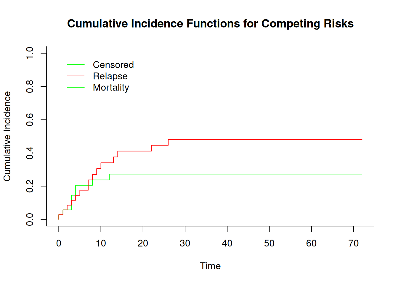


# Estimate the cumulative incidence functions fo each even type per group
cif <- cuminc(ftime = data_bmt$ftime, 
              fstatus = data_bmt$status, 
              group = data_bmt$dis) # Estimates will calculated within groups

# Plot the CIFs for both event types using survminer package
ggcompetingrisks(cif, multiple_panels = FALSE, legend = "right")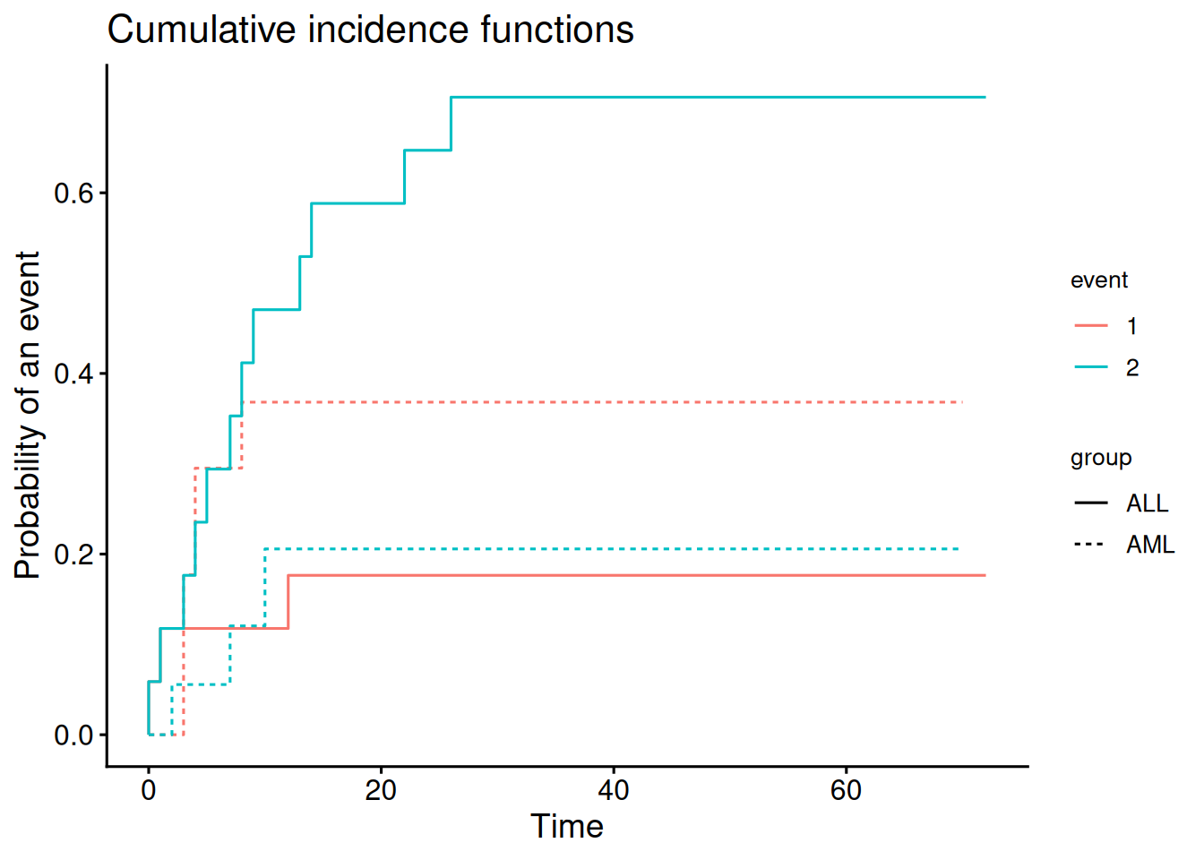


# Show Gray's test for equality of CIFs
print(cif$Tests)
##       stat          pv df
## 1 1.301635 0.253914871  1
## 2 7.082278 0.007784998  1

Gray’s test for equality of CIFs across groups (ALL vs. AML) is split across different types of events, here (Censored, Mortality, and Relapse).

For Censored, the p-value is small and suggest that there isa statistically significant difference in the CIF for censored events between the groups.
For Mortality, the p-value is greater than 0.05, suggesting that there is no statistically significant difference in the CIF for mortality between the groups.
For Relapse, the p-value is less than 0.05, indicating a statistically significant difference in the CIF for relapse between the groups.
The above suggest that the groups are behaving differently in terms of the time to relapse and censored events, but not for mortality.

24.5.2 Competing Risks Regression

adopted from https://www.nature.com/articles/bmt2009359

Suppose that the BMT study was extended to include more participants and additional covariates and now includes:

177 observations
Sex: gender of the individual
D: disease; 0 = ALL; 1 = AML
Phase: phase at transplant (Relapse, CR1, CR2, CR3)
Age: age at the beginning of follow-up
Status: 0 = censored; 1 = relapse; 2 = Transplant-related mortality
Source: source of stem cells (BM+PB, PB)
ftime: failure time

We are interested in modeling time to relapse in the presence of transplant-related death (competing event). We want to sutdy the effect on relapse of sex, disease type, phase at transplant, source of stem cells and age.

The data can be downloaded from here: data/data-bmtcrr.rds.

# load additional libraries
library(fastDummies)

# load data
data_bmtcrr <- readRDS("data/data-bmtcrr.rds")

# preview data
str(data_bmtcrr)
## 'data.frame':    177 obs. of  7 variables:
##  $ Sex   : Factor w/ 2 levels "F","M": 2 1 2 1 1 2 2 1 2 1 ...
##  $ D     : Factor w/ 2 levels "ALL","AML": 1 2 1 1 1 1 1 1 1 1 ...
##  $ Phase : Factor w/ 4 levels "CR1","CR2","CR3",..: 4 2 3 2 2 4 1 1 1 4 ...
##  $ Age   : int  48 23 7 26 36 17 7 17 26 8 ...
##  $ Status: int  2 1 0 2 2 2 0 2 0 1 ...
##  $ Source: Factor w/ 2 levels "BM+PB","PB": 1 1 1 1 1 1 1 1 1 1 ...
##  $ ftime : num  0.67 9.5 131.77 24.03 1.47 ...

# prepare matrix of covariates
# factor variables need to be coded as dummy variables
x_sex <- dummy_cols(data_bmtcrr$Sex) %>% dplyr::select(.data_F)
x_phase <- dummy_cols(data_bmtcrr$Phase) %>% dplyr::select(.data_CR1, .data_CR2, .data_CR3)
x_d <- dummy_cols(data_bmtcrr$D) %>% dplyr::select(.data_AML)
x_source <- dummy_cols(data_bmtcrr$Source) %>% dplyr::select(.data_PB)
x <- data.frame(age = data_bmtcrr$Age, sex = x_sex, x_d, x_phase, x_source)
colnames(x) <- c("age", "sex_F", "D_AML", "P:CR1", "P:CR2", "P:CR3", "source:PB")

# The first regression model for relapse can be produced by typing
mod1 <- crr(ftime = data_bmtcrr$ftime, 
            fstatus = data_bmtcrr$Status, 
            cov1 = x,
            failcode = 1) # code for relapse

summary(mod1)
## Competing Risks Regression
## 
## Call:
## crr(ftime = data_bmtcrr$ftime, fstatus = data_bmtcrr$Status, 
##     cov1 = x, failcode = 1)
## 
##              coef exp(coef) se(coef)      z p-value
## age       -0.0185     0.982   0.0119 -1.554  0.1200
## sex_F     -0.0352     0.965   0.2900 -0.122  0.9000
## D_AML     -0.4723     0.624   0.3054 -1.547  0.1200
## P:CR1     -1.1018     0.332   0.3764 -2.927  0.0034
## P:CR2     -1.0200     0.361   0.3558 -2.867  0.0041
## P:CR3     -0.7314     0.481   0.5766 -1.268  0.2000
## source:PB  0.9211     2.512   0.5530  1.666  0.0960
## 
##           exp(coef) exp(-coef)  2.5% 97.5%
## age           0.982      1.019 0.959 1.005
## sex_F         0.965      1.036 0.547 1.704
## D_AML         0.624      1.604 0.343 1.134
## P:CR1         0.332      3.009 0.159 0.695
## P:CR2         0.361      2.773 0.180 0.724
## P:CR3         0.481      2.078 0.155 1.490
## source:PB     2.512      0.398 0.850 7.426
## 
## Num. cases = 177
## Pseudo Log-likelihood = -267 
## Pseudo likelihood ratio test = 24.4  on 7 df,

The first part of the output shows for each term in the design matrix the estimated coefficient \(\hat{\beta}_j\), the relative risk \(\mathrm{exp}(\hat{\beta}_j)\), the standard error, the z-value and the corresponding P-value for assessing significance.

Here, Sex is not significant, followed by Age and D (disease type), whereas Source is only marginally significant. Phase is a factor with relapse as baseline, so each P-value provides a test for the difference of each level with respect to the baseline.

An overall P-value for Phase can be obtained through the Wald test via aod R package:

library(aod)
wald.test(mod1$var, mod1$coef, Terms = 4:6)
## Wald test:
## ----------
## 
## Chi-squared test:
## X2 = 14.0, df = 3, P(> X2) = 0.0029

The first argument to the function wald.test() is the estimated covariance matrix for the coefficients, followed by the vector of coefficients estimates, and the position of coefficients for which we want to assess significance. In our case, the P-value indicates that Phase is statistically significant.

The second part of the output for competing risks regression shows the relative risk for each term, and a 95% confidence interval. The relative risk or subdistribution hazard ratio for a categorical covariate is the ratio of subdistribution hazards for the actual group with respect to the baseline, with all other covariates being equal. If the covariate is continuous then the relative risk refers to the effect of a one unit increase in the covariate, with all other covariates being equal. In our data, exp(−0.0352)=0.965 is the relative risk of a woman with respect to a man, and exp(−0.0185)=0.982 is the relative risk for a 1 year increase in age.

The last part of the output shows the pseudo log-likelihood at maximum and the pseudo likelihood ratio test, that is, the difference in the objective function at the global null and at the final estimates. As this objective function is not a true likelihood, this test statistic is not asymptotically distributed as a χ2. As a consequence, model comparison based on likelihood ratio approach cannot be performed directly, but significance must be evaluated through simulations. However, a model selection criterion can be easily adopted as described in the following section.

For an example on model selection, model diagnostics or adding time-varying covariates in presence of competing events, please refer to the original tutorial article Scrucca, Santucci, and Aversa (2010) https://www.nature.com/articles/bmt2009359.