15 Introduction to linear models
15.1 Why linear models?
With linear models we can answer questions such as:
- is there a relationship between exposure and outcome, e.g. height and weight?
- how strong is the relationship between the two variables?
- what will be a predicted value of the outcome given a new set of exposure values?
- how accurately can we predict outcome?
- which variables are associated with the response, e.g. is it only height that explains weight or could it be height and age that are both associated with the response?
Code
data_diabetes %>%
  ggplot(aes(x = height, y = weight)) +
  geom_point() +
  geom_smooth(method = "lm", se = FALSE) +
  my.ggtheme +
  xlab("height [m]") +
  ylab("weight [kg]")
15.2 Statistical vs. deterministic relationship
Relationships in probability and statistics can generally be one of three things: deterministic, random, or statistical:
- a deterministic relationship involves an exact relationship between two variables, for instance Fahrenheit and Celsius degrees is defined by an equation \(Fahrenheit=\frac{9}{5}\cdot Celcius+32\)
- there is no relationship between variables in the random relationship, for instance number of succulents Olga buys and time of the year as Olga keeps buying succulents whenever she feels like it throughout the entire year
- a statistical relationship is a mixture of deterministic and random relationship, e.g. the savings that Olga has left in the bank account depend on Olga’s monthly salary income (deterministic part) and the money spent on buying succulents (random part)
15.3 What linear models are and are not
In an linear model we model (explain) the relationship between a single continuous variable \(Y\) and one or more variables \(X\). The \(X\) variables can be numerical, categorical or a mixture of both.
One very general form for the model would be: \[Y = f(X_1, X_2, \dots X_p) + \epsilon\] where \(f\) is some unknown function and \(\epsilon\) is the error in this representation.
For instance a simple linear regression through the origin is a simple linear model of the form \[Y_i = \beta \cdot x + \epsilon\] often used to express a relationship of one numerical variable to another, e.g. the calories burnt and the kilometers cycled.
Linear models can become quite advanced by including many variables, e.g. the calories burnt could be a function of the kilometers cycled, road incline and status of a bike, or the transformation of the variables, e.g. a function of kilometers cycled squared
Formally, linear models are a way of describing a response variable in terms of linear combination of predictor variables, i.e. expression constructed from a a set of terms by multiplying each term by a constant and/or adding the results.
For instance these are all models that can be constructed using linear combinations of predictors:

- \(Y_i = \alpha + \beta x_i + \gamma y_i + \epsilon_i\)
- \(Y_i = \alpha + \beta x_i^2 \epsilon\)
- \(Y_i = \alpha + \beta x_i^2 + \gamma x_i^3 + \epsilon\)
- \(Y_i = \beta_0 + \beta_1 x_i + \beta_2 x_i^2 + \beta_3 y_i + \beta_4 \sqrt {y_i} + \beta_5 x_i y_i + \epsilon\)
vs. an example of a non-linear model where parameter \(\beta\) appears in the exponent of \(x_i\)
- \(Y_i = \alpha + x_i^\beta + \epsilon\)
15.4 Terminology
There are many terms and notations used interchangeably:
- \(y\) is being called:
- response
- outcome
- dependent variable
- \(x\) is being called:
- exposure
- explanatory variable
- independent variable
- predictor
- covariate
15.5 Simple linear regression
- It is used to check the association between the numerical outcome and one numerical explanatory variable
- In practice, we are finding the best-fitting straight line to describe the relationship between the outcome and exposure
Example 15.1 (Weight and plasma volume) Let’s look at the example data containing body weight (kg) and plasma volume (liters) for eight healthy men to see what the best-fitting straight line is.
Example data:
weight <- c(58, 70, 74, 63.5, 62.0, 70.5, 71.0, 66.0) # body weight (kg)
plasma <- c(2.75, 2.86, 3.37, 2.76, 2.62, 3.49, 3.05, 3.12) # plasma volume (liters)

The equation for the red line is: \[Y_i=0.086 + 0.044 \cdot x_i \quad for \;i = 1 \dots 8\] and in general: \[Y_i=\alpha + \beta \cdot x_i \quad for \; i = 1 \dots n\]
- In other words, by finding the best-fitting straight line we are building a statistical model to represent the relationship between plasma volume (\(Y\)) and explanatory body weight variable (\(x\))
- If we were to use our model \(Y_i=0.086 + 0.044 \cdot x_i\) to find plasma volume given a weight of 58 kg (our first observation, \(i=1\)), we would notice that we would get \(Y=0.086 + 0.044 \cdot 58 = 2.638\), not exactly \(2.75\) as we have for our first man in our dataset that we started with, i.e. \(2.75 - 2.638 = 0.112 \neq 0\).
- We thus add to the above equation an error term to account for this and now we can write our simple regression model more formally as:
\[Y_i = \alpha + \beta \cdot x_i + \epsilon_i \tag{15.1}\] where:
- \(x\): is called: exposure variable, explanatory variable, dependent variable, predictor, covariate
- \(y\): is called: response, outcome, dependent variable
- \(\alpha\) and \(\beta\) are model coefficients
- and \(\epsilon_i\) is an error terms
15.6 Least squares
- in the above “body weight - plasma volume” example, the values of \(\alpha\) and \(\beta\) have just appeared
- in practice, \(\alpha\) and \(\beta\) values are unknown and we use data to estimate these coefficients, noting the estimates with a hat, \(\hat{\alpha}\) and \(\hat{\beta}\)
- least squares is one of the methods of parameters estimation, i.e. finding \(\hat{\alpha}\) and \(\hat{\beta}\)

Let \(\hat{y_i}=\hat{\alpha} + \hat{\beta}x_i\) be the prediction \(y_i\) based on the \(i\)-th value of \(x\):
- Then \(\epsilon_i = y_i - \hat{y_i}\) represents the \(i\)-th residual, i.e. the difference between the \(i\)-th observed response value and the \(i\)-th response value that is predicted by the linear model
- RSS, the residual sum of squares is defined as: \[RSS = \epsilon_1^2 + \epsilon_2^2 + \dots + \epsilon_n^2\] or equivalently as: \[RSS=(y_1-\hat{\alpha}-\hat{\beta}x_1)^2+(y_2-\hat{\alpha}-\hat{\beta}x_2)^2+...+(y_n-\hat{\alpha}-\hat{\beta}x_n)^2\]
- the least squares approach chooses \(\hat{\alpha}\) and \(\hat{\beta}\) to minimize the RSS. With some calculus, a good video explanation for the interested ones is here, we get Theorem 15.1
Theorem 15.1 (Least squares estimates for a simple linear regression) \[\hat{\beta} = \frac{S_{xy}}{S_{xx}}\] \[\hat{\alpha} = \bar{y}-\frac{S_{xy}}{S_{xx}}\cdot \bar{x}\]
where:
- \(\bar{x}\): mean value of \(x\)
- \(\bar{y}\): mean value of \(y\)
- \(S_{xx}\): sum of squares of \(X\) defined as \(S_{xx} = \displaystyle \sum_{i=1}^{n}(x_i-\bar{x})^2\)
- \(S_{yy}\): sum of squares of \(Y\) defined as \(S_{yy} = \displaystyle \sum_{i=1}^{n}(y_i-\bar{y})^2\)
- \(S_{xy}\): sum of products of \(X\) and \(Y\) defined as \(S_{xy} = \displaystyle \sum_{i=1}^{n}(x_i-\bar{x})(y_i-\bar{y})\)
Example 15.2 (Least squares) Let’s try least squares method to find coefficient estimates in the “body weight and plasma volume example”
# initial data
weight <- c(58, 70, 74, 63.5, 62.0, 70.5, 71.0, 66.0) # body weight (kg)
plasma <- c(2.75, 2.86, 3.37, 2.76, 2.62, 3.49, 3.05, 3.12) # plasma volume (liters)

# rename variables for convenience
x <- weight
y <- plasma

# mean values of x and y
x.bar <- mean(x)
y.bar <- mean(y)

# Sum of squares
Sxx <-  sum((x - x.bar)^2)
Sxy <- sum((x-x.bar)*(y-y.bar))

# Coefficient estimates
beta.hat <- Sxy / Sxx
alpha.hat <- y.bar - Sxy/Sxx*x.bar

# Print estimated coefficients alpha and beta
print(alpha.hat)
[1] 0.08572428print(beta.hat)[1] 0.04361534In R we can use lm(), the built-in function, to fit a linear regression model and we can replace the above code with one line
lm(plasma ~ weight)
Call:
lm(formula = plasma ~ weight)

Coefficients:
(Intercept)       weight
    0.08572      0.04362
15.7 The linear model describes an expected value
Another way to think about a linear regression model is that it describes the expected value of the outcome for a given value of the predictor.
For simple linear regression,
\[ E(Y\mid X=x)=\alpha+\beta x. \]
This means that for individuals with the same value \(X=x\), their observed outcomes \(Y\) do not all have to lie exactly on the regression line. Instead, the line describes their expected, or average, outcome.
An individual observation can therefore be written as
\[ Y_i = E(Y_i\mid X_i=x_i) + \epsilon_i \]
or, for the linear model,
\[ Y_i = \alpha+\beta x_i+\epsilon_i. \]
The error term \(\epsilon_i\) represents how much an individual observation differs from its expected value.
When we fit the model from a sample, we estimate this expected value by
\[ \hat{Y}_i=\hat{\alpha}+\hat{\beta}x_i, \]
and the difference between the observed and fitted value is the residual:
\[ e_i=Y_i-\hat{Y}_i. \]
Thus, the regression line describes how the expected outcome changes with the predictor, while individual observations vary around that expectation.
15.8 Intercept and Slope
- Linear regression gives us estimates of model coefficient \(Y_i = \alpha + \beta x_i + \epsilon_i\)
- \(\alpha\) is known as the intercept
- \(\beta\) is known as the slope

15.9 From simple regression to more general linear models
So far, we have considered simple linear regression, where a continuous outcome \(Y\) is described using one numerical predictor \(X\):
\[ Y_i = \beta_0 + \beta_1 x_i + \epsilon_i. \]
The same framework can be extended to include more than one predictor. For example, with two predictors:
\[ Y_i = \beta_0 + \beta_1 x_{1i} + \beta_2 x_{2i} + \epsilon_i. \]
More generally, a linear model with \(p\) predictors can be written as:
\[ Y_i = \beta_0 + \beta_1 x_{1i} + \beta_2 x_{2i} + \dots + \beta_p x_{pi} + \epsilon_i. \]
Each coefficient describes the contribution of one predictor to the expected outcome, while keeping the other predictors in the model constant.
For example, if body weight is modelled using height and age,
\[E(\text{weight}\mid\text{height},\text{age})= \beta_0 + \beta_1\text{height} + \beta_2\text{age}, \]
then \(\beta_1\) describes the expected difference in weight associated with a one-unit difference in height for individuals of the same age.
Predictors in a linear model do not have to be numerical. They can also be categorical, such as treatment group, sex, genotype or experimental condition. This allows the same linear-model framework to describe both relationships between continuous variables and differences between groups.
We will look at how numerical and categorical predictors, and combinations of several predictors, are used in practice in the next session.
15.10 Hypothesis testing
Is there a relationship between the response and the predictor?
- the calculated \(\hat{\alpha}\) and \(\hat{\beta}\) are estimates of the population values of the intercept and slope and are therefore subject to sampling variation
- their precision is measured by their estimated standard errors,
e.s.e(\(\hat{\alpha}\)) ande.s.e(\(\hat{\beta}\)) - these estimated standard errors are used in hypothesis testing and in constructing confidence and prediction intervals
The most common hypothesis test involves testing the null hypothesis of:
- \(H_0:\) There is no relationship between \(X\) and \(Y\)
- versus the
alternative hypothesis\(H_a:\) there is some relationship between \(X\) and \(Y\)
Mathematically, this corresponds to testing:
- \(H_0: \beta=0\)
- versus \(H_a: \beta\neq0\)
- since if \(\beta=0\) then the model \(Y_i=\alpha+\beta x_i + \epsilon_i\) reduces to \(Y=\alpha + \epsilon_i\)
Under the null hypothesis \(H_0: \beta = 0\) 
- \(n\) is number of observations
- \(p\) is number of model parameters
- \(\frac{\hat{\beta}-\beta}{e.s.e(\hat{\beta})}\) is the ratio of the departure of the estimated value of a parameter, \(\hat\beta\), from its hypothesized value, \(\beta\), to its standard error, called
t-statistics - the
t-statisticsfollows Student’s t distribution with \(n-p\) degrees of freedom
Example 15.3 (Hypothesis testing) Let’s look again at our example data. This time we will not only fit the linear regression model but also look a bit more closely at the R summary of the model
weight <- c(58, 70, 74, 63.5, 62.0, 70.5, 71.0, 66.0) # body weight (kg)
plasma <- c(2.75, 2.86, 3.37, 2.76, 2.62, 3.49, 3.05, 3.12) # plasma volume (liters)

model <- lm(plasma ~ weight)
print(summary(model))
Call:
lm(formula = plasma ~ weight)

Residuals:
     Min       1Q   Median       3Q      Max
-0.27880 -0.14178 -0.01928  0.13986  0.32939

Coefficients:
            Estimate Std. Error t value Pr(>|t|)
(Intercept)  0.08572    1.02400   0.084   0.9360
weight       0.04362    0.01527   2.857   0.0289 *
---
Signif. codes:  0 '***' 0.001 '**' 0.01 '*' 0.05 '.' 0.1 ' ' 1

Residual standard error: 0.2188 on 6 degrees of freedom
Multiple R-squared:  0.5763,    Adjusted R-squared:  0.5057
F-statistic: 8.16 on 1 and 6 DF, p-value: 0.02893- Under
Estimatewe see estimates of our model coefficients, \(\hat{\alpha}\) (intercept) and \(\hat{\beta}\) (slope, here weight), followed by their estimated standard errors,Std. Errors - If we were to test if there is an association between weight and plasma volume we would write under the null hypothesis \(H_0: \beta = 0\) \[\frac{\hat{\beta}-\beta}{e.s.e(\hat{\beta})} = \frac{0.04362-0}{0.01527} = 2.856582\]
- and we would compare
t-statisticstoStudent's t distributionwith \(n-p = 8 - 2 = 6\) degrees of freedom (as we have 8 observations and two model parameters, \(\alpha\) and \(\beta\)) - we can use Student’s t distribution table or R code to obtain the associated P-value
2*pt(2.856582, df=6, lower=F)[1] 0.02893095- here the observed t-statistics is large and therefore yields a small P-value, meaning that there is sufficient evidence to reject null hypothesis in favor of the alternative and conclude that there is a significant association between weight and plasma volume
15.11 Overall model test: the F-test
The summary() output also reports an F-statistic and its corresponding P-value. The F-test evaluates the linear model as a whole.
For a linear model with several predictors,
\[ Y_i = \beta_0 + \beta_1x_{1i} + \cdots + \beta_{p-1}x_{(p-1)i} + \epsilon_i, \]
the overall null hypothesis is
\[ H_0:\beta_1=\beta_2=\cdots=\beta_{p-1}=0. \]
In other words, under the null hypothesis none of the predictors contributes to explaining variation in the response, and the model reduces to an intercept-only model.
The F-statistic compares the variation explained by the regression model with the variation left unexplained by the model:
\[ F = \frac{\text{explained variation per degree of freedom}} {\text{unexplained variation per degree of freedom}}. \]
Under the null hypothesis, the F-statistic follows an F-distribution with
\[ (p-1,\; n-p) \]
degrees of freedom, where \(n\) is the number of observations and \(p\) is the number of estimated model parameters, including the intercept.
For our plasma-volume example,
Code
weight <- c(58, 70, 74, 63.5, 62.0, 70.5, 71.0, 66.0)
plasma <- c(2.75, 2.86, 3.37, 2.76, 2.62, 3.49, 3.05, 3.12)

model <- lm(plasma ~ weight)
summary(model)
Call:
lm(formula = plasma ~ weight)

Residuals:
     Min       1Q   Median       3Q      Max
-0.27880 -0.14178 -0.01928  0.13986  0.32939

Coefficients:
            Estimate Std. Error t value Pr(>|t|)
(Intercept)  0.08572    1.02400   0.084   0.9360
weight       0.04362    0.01527   2.857   0.0289 *
---
Signif. codes:  0 '***' 0.001 '**' 0.01 '*' 0.05 '.' 0.1 ' ' 1

Residual standard error: 0.2188 on 6 degrees of freedom
Multiple R-squared:  0.5763,    Adjusted R-squared:  0.5057
F-statistic:  8.16 on 1 and 6 DF,  p-value: 0.02893
Here we have \(n=8\) observations and \(p=2\) model parameters, the intercept \(\alpha\) and slope \(\beta\). Therefore,
\[ F \sim F_{1,6} \]
under the null hypothesis.
The P-value is the probability, under \(H_0\), of observing an F-statistic at least as large as the one obtained:
\[ P(F_{1,6} \geq 8.16) \approx 0.029. \]
Thus, there is sufficient evidence to reject the null hypothesis and conclude that the model containing weight explains more variation in plasma volume than an intercept-only model.
In simple linear regression, with only one predictor, the overall F-test tests exactly the same hypothesis as the t-test for the slope:
\[ H_0:\beta=0. \]
In this case,
\[ F=t^2, \]
so the two tests give the same P-value. With several predictors, the F-test is useful because it tests whether the predictors are jointly associated with the response.
15.12 Vector-matrix notations
While in simple linear regression it is feasible to arrive at the parameters estimates using calculus in more realistic settings of multiple regression, with more than one explanatory variable in the model, it is more efficient to use vectors and matrices to define the regression model.
Let’s rewrite our simple linear regression model \(Y_i = \alpha + \beta_i + \epsilon_i \quad i=1,\dots n\) into vector-matrix notation in 6 steps.
First we rename our \(\alpha\) to \(\beta_0\) and \(\beta\) to \(\beta_1\) as it is easier to keep tracking the number of model parameters this way
Then we notice that we actually have \(n\) equations such as: \[y_1 = \beta_0 + \beta_1 x_1 + \epsilon_1\] \[y_2 = \beta_0 + \beta_1 x_2 + \epsilon_2\] \[y_3 = \beta_0 + \beta_1 x_3 + \epsilon_3\] \[\dots\] \[y_n = \beta_0 + \beta_1 x_n + \epsilon_n\]
We group all \(Y_i\) and \(\epsilon_i\) into column vectors: \(\mathbf{Y}=\begin{bmatrix} y_1 \\ y_2 \\ \vdots \\ y_{n} \end{bmatrix}\) and \(\boldsymbol\epsilon=\begin{bmatrix} \epsilon_1 \\ \epsilon_2 \\ \vdots \\ \epsilon_{n} \end{bmatrix}\)
We stack two parameters \(\beta_0\) and \(\beta_1\) into another column vector:\[\boldsymbol\beta=\begin{bmatrix} \beta_0 \\ \beta_1 \end{bmatrix}\]
We append a vector of ones with the single predictor for each \(i\) and create a matrix with two columns called design matrix \[\mathbf{X}=\begin{bmatrix} 1 & x_1 \\ 1 & x_2 \\ \vdots & \vdots \\ 1 & x_{n} \end{bmatrix}\]
We write our linear model in a vector-matrix notations as: \[\mathbf{Y} = \mathbf{X}\boldsymbol\beta + \boldsymbol\epsilon\]
Definition 15.1 (vector matrix form of the linear model) The vector-matrix representation of a linear model with \(p-1\) predictors can be written as \[\mathbf{Y} = \mathbf{X}\boldsymbol\beta + \boldsymbol\epsilon\]
where:
- \(\mathbf{Y}\) is \(n \times1\) vector of observations
- \(\mathbf{X}\) is \(n \times p\) design matrix
- \(\boldsymbol\beta\) is \(p \times1\) vector of parameters
- \(\boldsymbol\epsilon\) is \(n \times1\) vector of vector of random errors, indepedent and identically distributed (i.i.d) N(0, \(\sigma^2\))
In full, the above vectors and matrix have the form:
\(\mathbf{Y}=\begin{bmatrix} y_1 \\ y_2 \\ \vdots \\ y_{n} \end{bmatrix}\) \(\boldsymbol\beta=\begin{bmatrix} \beta_0 \\ \beta_1 \\ \vdots \\ \beta_{p} \end{bmatrix}\) \(\boldsymbol\epsilon=\begin{bmatrix} \epsilon_1 \\ \epsilon_2 \\ \vdots \\ \epsilon_{n} \end{bmatrix}\) \(\mathbf{X}=\begin{bmatrix} 1 & x_{1,1} & \dots & x_{1,p-1} \\ 1 & x_{2,1} & \dots & x_{2,p-1} \\ \vdots & \vdots & \vdots & \vdots \\ 1 & x_{n,1} & \dots & x_{n,p-1} \end{bmatrix}\)
Theorem 15.2 (Least squares in vector-matrix notation) The least squares estimates for a linear regression of the form: \[\mathbf{Y} = \mathbf{X}\boldsymbol\beta + \boldsymbol\epsilon\]
is given by: \[\hat{\mathbf{\beta}}= (\mathbf{X}^T\mathbf{X})^{-1}\mathbf{X}^T\mathbf{Y}\]
Example 15.4 (vector-matrix-notation) Following the above definition we can write the “weight - plasma volume model” as: \[\mathbf{Y} = \mathbf{X}\boldsymbol\beta + \boldsymbol\epsilon\] where:
\(\mathbf{Y}=\begin{bmatrix} 2.75 \\ 2.86 \\ 3.37 \\ 2.76 \\ 2.62 \\ 3.49 \\ 3.05 \\ 3.12 \end{bmatrix}\)
\(\boldsymbol\beta=\begin{bmatrix} \beta_0 \\ \beta_1 \end{bmatrix}\) \(\boldsymbol\epsilon=\begin{bmatrix} \epsilon_1 \\ \epsilon_2 \\ \vdots \\ \epsilon_{8} \end{bmatrix}\) \(\mathbf{X}=\begin{bmatrix} 1 & 58.0 \\ 1 & 70.0 \\ 1 & 74.0 \\ 1 & 63.5 \\ 1 & 62.0 \\ 1 & 70.5 \\ 1 & 71.0 \\ 1 & 66.0 \\ \end{bmatrix}\)
and we can estimate model parameters using \(\hat{\mathbf{\beta}}= (\mathbf{X}^T\mathbf{X})^{-1}\mathbf{X}^T\mathbf{Y}\).
We can do it by hand or in R as follows:
n <- length(plasma) # no. of observation
Y <- as.matrix(plasma, ncol=1)
X <- cbind(rep(1, length=n), weight)
X <- as.matrix(X)

# print Y and X to double-check that the format is according to the definition
print(Y)
[,1]
[1,] 2.75
[2,] 2.86
[3,] 3.37
[4,] 2.76
[5,] 2.62
[6,] 3.49
[7,] 3.05
[8,] 3.12print(X) weight
[1,] 1 58.0
[2,] 1 70.0
[3,] 1 74.0
[4,] 1 63.5
[5,] 1 62.0
[6,] 1 70.5
[7,] 1 71.0
[8,] 1 66.0# least squares estimate
# solve() finds inverse of matrix
beta.hat <- solve(t(X)%*%X)%*%t(X)%*%Y
print(beta.hat) [,1]
0.08572428
weight 0.0436153415.13 Confidence intervals and prediction intervals
- when we estimate coefficients we can also find their confidence intervals, typically 95% confidence intervals, i.e. a range of values that contain the true unknown value of the parameter
- we can also use linear regression models to predict the response value given a new observation and find prediction intervals. Here, we look at any specific value of \(x_i\), and find an interval around the predicted value \(y_i'\) for \(x_i\) such that there is a 95% probability that the real value of y (in the population) corresponding to \(x_i\) is within this interval
Example 15.5 (Prediction and intervals) Let’s:
- find confidence intervals for our coefficient estimates
- predict plasma volume for a men weighting 60 kg
- find prediction interval
- plot original data, fitted regression model, predicted observation and prediction interval
# fit regression model
model <- lm(plasma ~ weight)
print(summary(model))
Call:
lm(formula = plasma ~ weight)

Residuals:
     Min       1Q   Median       3Q      Max
-0.27880 -0.14178 -0.01928  0.13986  0.32939

Coefficients:
            Estimate Std. Error t value Pr(>|t|)
(Intercept)  0.08572    1.02400   0.084   0.9360
weight       0.04362    0.01527   2.857   0.0289 *
---
Signif. codes:  0 '***' 0.001 '**' 0.01 '*' 0.05 '.' 0.1 ' ' 1

Residual standard error: 0.2188 on 6 degrees of freedom
Multiple R-squared:  0.5763,    Adjusted R-squared:  0.5057
F-statistic:  8.16 on 1 and 6 DF,  p-value: 0.02893
# find confidence intervals for the model coefficients
confint(model) 2.5 % 97.5 %
(Intercept) -2.419908594 2.59135716
weight 0.006255005 0.08097567# predict plasma volume for a new observation of 60 kg
# we have to create data frame with a variable name matching the one used to build the model
new.obs <- data.frame(weight = 60)
predict(model, newdata = new.obs) 1
2.702645 # find prediction intervals
prediction.interval <- predict(model, newdata = new.obs, interval = "prediction")
print(prediction.interval) fit lwr upr
1 2.702645 2.079373 3.325916# plot the original data, fitted regression and predicted value
plot(weight, plasma, pch=19, xlab="weight [kg]", ylab="plasma [l]", ylim=c(2,4))
lines(weight, model$fitted.values, col="red") # fitted model in red
points(new.obs, predict(model, newdata = new.obs), pch=19, col="blue") # predicted value at 60kg
segments(60, prediction.interval[2], 60, prediction.interval[3], lty = 3) # add prediction interval
15.14 Assessing model fit
- Earlier we learned how to estimate parameters in a liner model using least squares estimation.
- Now we will consider how to assess the goodness of fit of a model, i.e. how well does the model explain our data.
- We do that by calculating the amount of variability in the response that is explained by the model.
\(R^2\): summary of the fitted model
- considering a simple linear regression, the simplest model, Model 0, we could consider fitting is \[Y_i = \beta_0+ \epsilon_i\] that corresponds to a line that run through the data but lies parallel to the horizontal axis
- in our plasma volume example that would correspond the mean value of plasma volume being predicted for any value of weight (in purple)

- TSS, denoted Total corrected sum-of-squares is the residual sum-of-squares for Model 0 \[S(\hat{\beta_0}) = TSS = \sum_{i=1}^{n}(y_i - \bar{y})^2 = S_{yy}\] corresponding the to the sum of squared distances to the purple line

- Fitting Model 1 of the form \[Y_i = \beta_0 + \beta_1x + \epsilon_i\] we have earlier defined
- RSS, the residual sum-of-squares as: \[RSS = \displaystyle \sum_{i=1}^{n}(y_i - \{\hat{\beta_0} + \hat{\beta}_1x_{1i} + \dots + \hat{\beta}_px_{pi}\}) = \sum_{i=1}^{n}(y_i - \hat{y_i})^2\]
- that corresponds to the squared distances between the observed values \(y_i, \dots,y_n\) to fitted values \(\hat{y_1}, \dots \hat{y_n}\), i.e. distances to the red fitted line
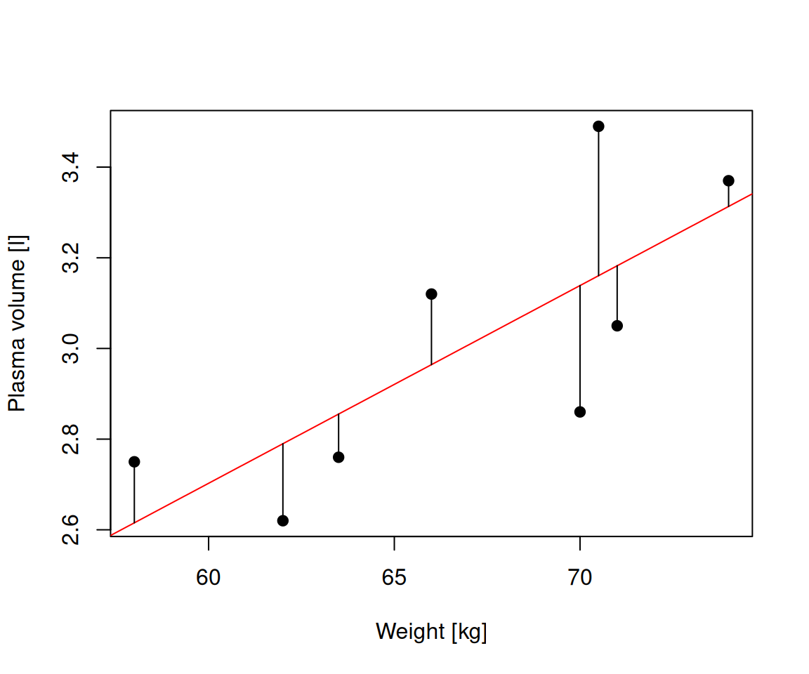
Definition 15.2 (\(R^2\)) A simple but useful measure of model fit is given by \[R^2 = 1 - \frac{RSS}{TSS}\] where:
- RSS is the residual sum-of-squares for Model 1, the fitted model of interest
- TSS is the sum of squares of the null model
- \(R^2\) quantifies how much of a drop in the residual sum-of-squares is accounted for by fitting the proposed model
- \(R^2\) is also referred as coefficient of determination
- It is expressed on a scale, as a proportion (between 0 and 1) of the total variation in the data
- Values of \(R^2\) approaching 1 indicate the model to be a good fit
- Values of \(R^2\) less than 0.5 suggest that the model gives rather a poor fit to the data
\(R^2\) and correlation coefficient
Theorem 15.3 (\(R^2\)) In the case of simple linear regression:
Model 1: \(Y_i = \beta_0 + \beta_1x + \epsilon_i\) \[R^2 = r^2\] where:
- \(R^2\) is the coefficient of determination
- \(r^2\) is the sample correlation coefficient
\(R^2(adj)\)
- in the case of multiple linear regression, where there is more than one explanatory variable in the model
- we are using the adjusted version of \(R^2\) to assess the model fit
- as the number of explanatory variables increase, \(R^2\) also increases
- \(R^2(adj)\) takes this into account, i.e. adjusts for the fact that there is more than one explanatory variable in the model
Theorem 15.4 (\(R^2(adj)\)) For any multiple linear regression \[Y_i = \beta_0 + \beta_1x_{1i} + \dots + \beta_{p-1}x_{(p-1)i} + \epsilon_i\] \(R^2(adj)\) is defined as \[R^2(adj) = 1-\frac{\frac{RSS}{n-p-1}}{\frac{TSS}{n-1}}\] where
- \(p\) is the number of independent predictors, i.e. the number of variables in the model, excluding the constant
\(R^2(adj)\) can also be calculated from \(R^2\): \[R^2(adj) = 1 - (1-R^2)\frac{n-1}{n-p-1}\]
15.15 The assumptions of a linear model
Up until now we were fitting models and discussed how to assess the model fit. Before making use of a fitted model for explanation or prediction, it is wise to check that the model provides an adequate description of the data. Informally we have been using box plots and scatter plots to look at the data. There are however formal definitions of the assumptions.
Assumption A: The deterministic part of the model captures all the non-random structure in the data
- This implies that the mean of the errors \(\epsilon_i\) is zero.
- Tt applies only over the range of explanatory variables.
Assumption B: the scale of variability of the errors is constant at all values of the explanatory variables
- Practically we are looking at whether the observations are equally spread on both side of the regression line.
Assumption C: the errors are independent
- Broadly speaking this means that knowledge of errors attached to one observation does not give us any information about the error attached to another.
Assumptions D: the errors are normally distributed
- This will allow us to describe the variation in the model’s parameters estimates and therefore make inferences about the population from which our sample was taken.
Assumption E: the values of the explanatory variables are recorded without error
- This one is not possible to check via examining the data, instead we have to consider the nature of the experiment.
15.15.1 Checking assumptions
Residuals, \(\hat{\epsilon_i} = y_i - \hat{y_i}\) are the main ingredient to check model assumptions. We use plots such as:
- Histograms or normal probability plots of \(\hat{\epsilon_i}\)
- useful to check the assumption of normality
- Plots of \(\hat{\epsilon_i}\) versus the fitted values \(\hat{y_i}\)
- used to detect changes in error variance
- used to check if the mean of the errors is zero
- Plots of \(\hat{\epsilon_i}\) vs. an explanatory variable \(x_{ij}\)
- this helps to check that the variable \(x_j\) has a linear relationship with the response variable
- Plots of \(\hat{\epsilon_i}\) vs. an explanatory variable \(x_{kj}\) that is not in the model
- this helps to check whether the additional variable \(x_k\) might have a relationship with the response variable
- Plots of \(\hat{\epsilon_i}\) in the order of the observations were collected
- this is useful to check whether errors might be correlated over time
Let’s fit a simple model to predict BMI given waist for the diabetes study and see if the model meets the assumptions of linear models.
# fit simple linear regression model
model <- lm(BMI ~ waist, data = data_diabetes)

# plot diagnostic plots of the linear model
# by default plot(model) calls four diagnostics plots
# par() divides plot window in 2 x 2 grid
par(mfrow=c(2,2))
plot(model)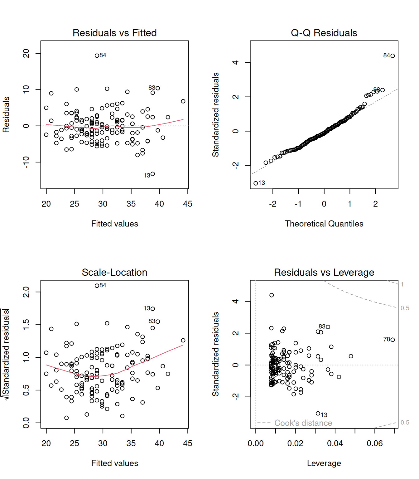
- The residual plots provides examples of a situation where the assumptions appear to be met.
- The linear regression appears to describe data quite well.
- There is no obvious trend of any kind in the residuals vs. fitted values (the shape is scattered) with potential few outliers that we may want to decided to exclude later.
- Points lie reasonably well along the line in the normal probability plot, hence normality appears to be met.
Examples of assumptions not being met
The following simulated examples show some typical patterns that may appear in diagnostic plots when linear model assumptions are violated.
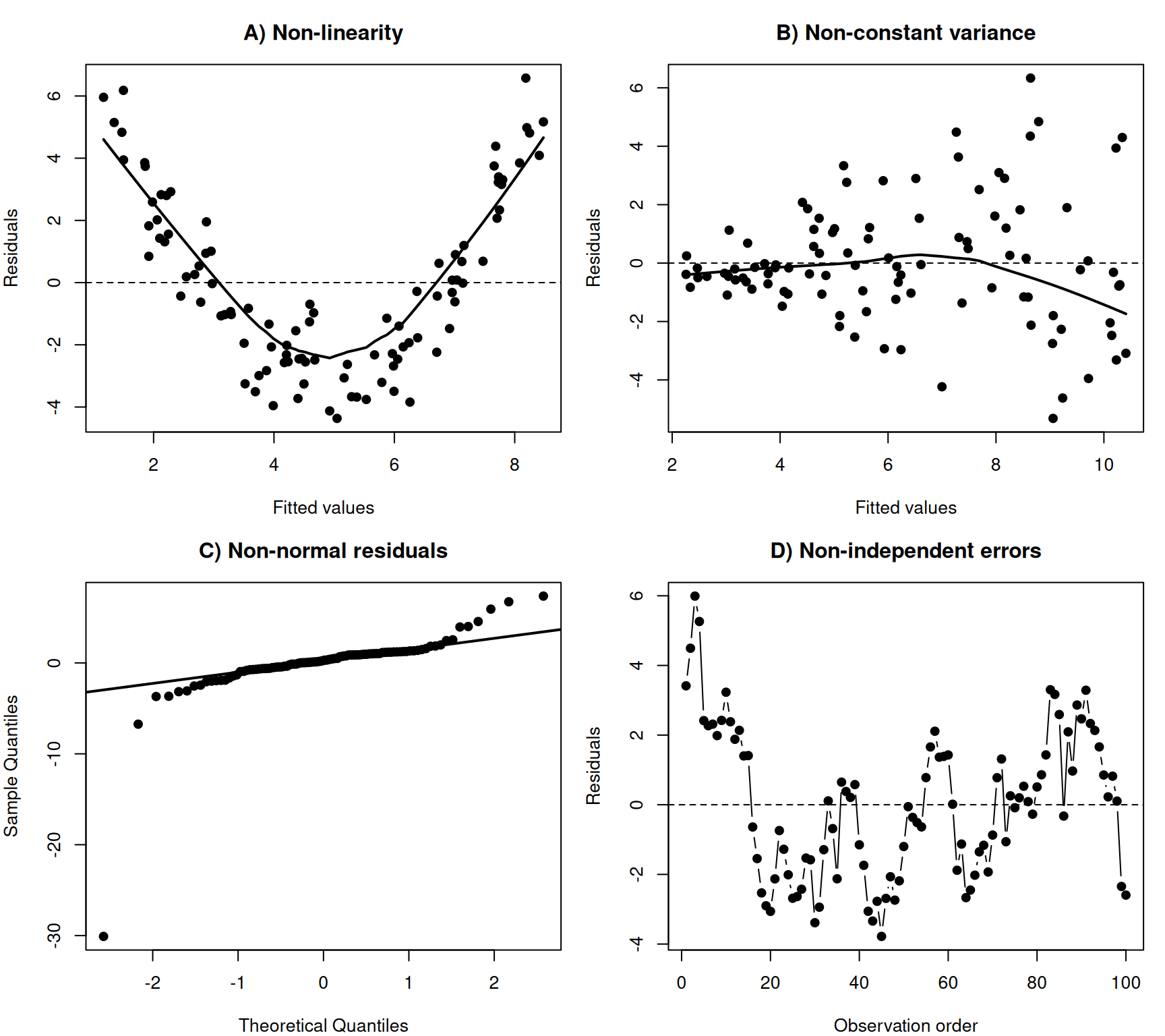
Typical warning signs include:
- Non-linearity: a systematic curved pattern remains in the residuals.
- Non-constant variance: the spread of residuals changes with the fitted values, often forming a funnel shape.
- Non-normality: residuals deviate systematically from the straight line in the normal Q–Q plot.
- Non-independence: neighbouring observations tend to have similar residuals, producing runs or other structure when residuals are plotted in observation order.
The exact appearance will vary between data sets. Diagnostic plots should therefore be interpreted as tools for identifying systematic patterns, rather than as formal pass/fail tests.
15.16 Influential observations
- Sometimes individual observations can exert a great deal of influence on the fitted model.
- One routine way of checking for this is to fit the model \(n\) times, missing out each observation in turn.
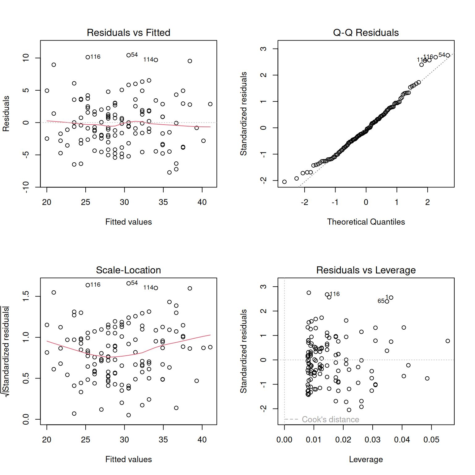
- If we removed i-th observation and compared the fitted value from the full model, say \(\hat{y_j}\) to those obtained by removing this point, denoted \(\hat{y_{j(i)}}\) then
- observations with a high Cook’s distance (measuring the effect of deleting a given observation) could be influential.
Let’s remove some observation with higher Cook’s distance from protein data set, re-fit our model and compare the diagnostics plots
# observations to be removed (based on Residuals vs. Leverage plot)
obs <- c(13, 78, 83, 84)

# fit models removing observations
data_diabetes_flr <- data_diabetes[-obs, ]

model_flr <- lm(BMI ~ waist, data = data_diabetes_flr)

# plot diagnostics plot
par(mfrow=c(2,2))
plot(model_flr)