Exercises (Lasso)

Data for exercises are on Canvas under Files -> data_exercises –> linear-models

Exercise 1 (Lasso) Follow and try to run the code below for fitting Lasso model to predict BMI given all the numerical variables in the diabetes data set.

Exercise 2 (MAE)  

• Add a code to calculate MAE, Mean Absolute Error to get a metric of model performance.
• Adjust the code, to get the best Lasso model again, but now exclude weight from the predictors. What value of MEA are you getting for this model, and what does it mean?

Exercise 3 (Logistic Lasso) Adjust the original code to model probability of becoming obese. You can define obesity as BMI > 30. Evaluate the final model using overall accuracy.

Load data & reformat data

# load libraries
library(tidyverse)
library(glmnet)
library(caret)
library(splitTools)

# import raw data
input_diabetes <- read_csv("data/data-diabetes.csv")

# preview data
glimpse(input_diabetes)

Rows: 403
Columns: 19
$ id       <dbl> 1000, 1001, 1002, 1003, 1005, 1008, 1011, 1015, 1016, 1022, 1…
$ chol     <dbl> 203, 165, 228, 78, 249, 248, 195, 227, 177, 263, 242, 215, 23…
$ stab.glu <dbl> 82, 97, 92, 93, 90, 94, 92, 75, 87, 89, 82, 128, 75, 79, 76, …
$ hdl      <dbl> 56, 24, 37, 12, 28, 69, 41, 44, 49, 40, 54, 34, 36, 46, 30, 4…
$ ratio    <dbl> 3.6, 6.9, 6.2, 6.5, 8.9, 3.6, 4.8, 5.2, 3.6, 6.6, 4.5, 6.3, 6…
$ glyhb    <dbl> 4.31, 4.44, 4.64, 4.63, 7.72, 4.81, 4.84, 3.94, 4.84, 5.78, 4…
$ location <chr> "Buckingham", "Buckingham", "Buckingham", "Buckingham", "Buck…
$ age      <dbl> 46, 29, 58, 67, 64, 34, 30, 37, 45, 55, 60, 38, 27, 40, 36, 3…
$ gender   <chr> "female", "female", "female", "male", "male", "male", "male",…
$ height   <dbl> 62, 64, 61, 67, 68, 71, 69, 59, 69, 63, 65, 58, 60, 59, 69, 6…
$ weight   <dbl> 121, 218, 256, 119, 183, 190, 191, 170, 166, 202, 156, 195, 1…
$ frame    <chr> "medium", "large", "large", "large", "medium", "large", "medi…
$ bp.1s    <dbl> 118, 112, 190, 110, 138, 132, 161, NA, 160, 108, 130, 102, 13…
$ bp.1d    <dbl> 59, 68, 92, 50, 80, 86, 112, NA, 80, 72, 90, 68, 80, NA, 66, …
$ bp.2s    <dbl> NA, NA, 185, NA, NA, NA, 161, NA, 128, NA, 130, NA, NA, NA, N…
$ bp.2d    <dbl> NA, NA, 92, NA, NA, NA, 112, NA, 86, NA, 90, NA, NA, NA, NA, …
$ waist    <dbl> 29, 46, 49, 33, 44, 36, 46, 34, 34, 45, 39, 42, 35, 37, 36, 3…
$ hip      <dbl> 38, 48, 57, 38, 41, 42, 49, 39, 40, 50, 45, 50, 41, 43, 40, 4…
$ time.ppn <dbl> 720, 360, 180, 480, 300, 195, 720, 1020, 300, 240, 300, 90, 7…

# run basic feature engieering of the data
# exclude bp.2s, pb.2d due to large number of missing data 
# create BMI based on weight and height
# keep only numerical variables
# keep samples for which none missing data is present (complete case analysis)

# define numerical predictors
pred_numeric <- c("chol", "stab.glu", "hdl", "ratio", "glyhb", "age", "weight", "bp.1s", "bp.1d", "waist", "hip", "time.ppn")

# and only numerical predictors
conv_factor <- 703 # conversion factor to calculate BMI from inches and pounds BMI = weight (lb) / [height (in)]2 x 703
data_diabetes <- input_diabetes %>%
  mutate(BMI = weight / height^2 * 703, BMI = round(BMI, 2)) %>%
  relocate(BMI, .after = id) %>%
  dplyr::select(-bp.2s, -bp.2d) %>%
  select(all_of(c("BMI", pred_numeric))) %>%
  na.omit()
  
# preview reformatted data
glimpse(data_diabetes)

Rows: 375
Columns: 13
$ BMI      <dbl> 22.13, 37.42, 48.37, 18.64, 27.82, 26.50, 28.20, 24.51, 35.78…
$ chol     <dbl> 203, 165, 228, 78, 249, 248, 195, 177, 263, 242, 215, 238, 19…
$ stab.glu <dbl> 82, 97, 92, 93, 90, 94, 92, 87, 89, 82, 128, 75, 76, 83, 78, …
$ hdl      <dbl> 56, 24, 37, 12, 28, 69, 41, 49, 40, 54, 34, 36, 30, 47, 38, 6…
$ ratio    <dbl> 3.6, 6.9, 6.2, 6.5, 8.9, 3.6, 4.8, 3.6, 6.6, 4.5, 6.3, 6.6, 6…
$ glyhb    <dbl> 4.31, 4.44, 4.64, 4.63, 7.72, 4.81, 4.84, 4.84, 5.78, 4.77, 4…
$ age      <dbl> 46, 29, 58, 67, 64, 34, 30, 45, 55, 60, 38, 27, 36, 33, 50, 2…
$ weight   <dbl> 121, 218, 256, 119, 183, 190, 191, 166, 202, 156, 195, 170, 1…
$ bp.1s    <dbl> 118, 112, 190, 110, 138, 132, 161, 160, 108, 130, 102, 130, 1…
$ bp.1d    <dbl> 59, 68, 92, 50, 80, 86, 112, 80, 72, 90, 68, 80, 66, 90, 100,…
$ waist    <dbl> 29, 46, 49, 33, 44, 36, 46, 34, 45, 39, 42, 35, 36, 37, 37, 3…
$ hip      <dbl> 38, 48, 57, 38, 41, 42, 49, 40, 50, 45, 50, 41, 40, 41, 43, 3…
$ time.ppn <dbl> 720, 360, 180, 480, 300, 195, 720, 300, 240, 300, 90, 720, 22…

split data and scale

# split data into train (70%) and test (30%)
set.seed(123)
inds <- partition(data_diabetes$BMI, p = c(train = 0.7, test = 0.3))

data_train <- data_diabetes %>%
  slice(inds$train)

data_test <- data_diabetes %>%
  slice(inds$test)

# standardize variables
# Note: the correct approach is to scale the non-test data (train) 
# and then scale the test data using the parameters of the train data (e.g. mean or sd)
# Here we will use preProcess() function from caret package to do that
# We do not scale response (BMI)

scaling <- preProcess(data_train[, pred_numeric], method = c("center", "scale"))
data_train[, pred_numeric] <- predict(scaling, data_train[, pred_numeric])
data_test[, pred_numeric] <- predict(scaling, data_test[, pred_numeric])

# preview scaled data
glimpse(data_train)

Rows: 258
Columns: 13
$ BMI      <dbl> 48.37, 27.82, 26.50, 28.20, 40.75, 33.20, 27.02, 26.12, 24.90…
$ chol     <dbl> 0.4524462, 0.9164540, 0.8943584, -0.2767090, 0.1652032, 0.673…
$ stab.glu <dbl> -0.28652567, -0.32418417, -0.24886718, -0.28652567, 0.3913272…
$ hdl      <dbl> -0.749786859, -1.261997828, 1.071407700, -0.522137539, -0.920…
$ ratio    <dbl> 0.89155394, 2.35907876, -0.52161816, 0.13061530, 0.94590692, …
$ glyhb    <dbl> -0.42464460, 0.91116765, -0.35091467, -0.33790342, -0.2815218…
$ age      <dbl> 0.70202683, 1.05915385, -0.72648126, -0.96456594, -0.48839658…
$ weight   <dbl> 1.8615300087, 0.1191556829, 0.2862326730, 0.3101008145, 0.405…
$ bp.1s    <dbl> 2.23602108, 0.03429933, -0.21974548, 1.00813780, -1.48996957,…
$ bp.1d    <dbl> 0.62214432, -0.24471383, 0.18871524, 2.06690792, -1.11157199,…
$ waist    <dbl> 1.8500049, 1.0090936, -0.3363645, 1.3454581, 0.6727291, -0.50…
$ hip      <dbl> 2.42867737, -0.36396335, -0.18942330, 1.03235701, 1.20689706,…
$ time.ppn <dbl> -0.5033145, -0.1207312, -0.4554916, 1.2183102, -0.7902519, 1.…

glimpse(data_test)

Rows: 117
Columns: 13
$ BMI      <dbl> 22.13, 37.42, 18.64, 24.51, 35.78, 25.96, 30.45, 21.63, 32.61…
$ chol     <dbl> -0.09994410, -0.93957728, -2.86189536, -0.67442996, 1.2257925…
$ stab.glu <dbl> -0.47481814, -0.19237944, -0.26769642, -0.38067191, -0.343013…
$ hdl      <dbl> 0.331547411, -1.489647148, -2.172595108, -0.066838899, -0.579…
$ ratio    <dbl> -0.52161816, 1.27202352, 1.05461237, -0.52161816, 1.10896509,…
$ glyhb    <dbl> -0.56776732, -0.51138558, -0.42898155, -0.33790342, 0.0697795…
$ age      <dbl> -0.01222722, -1.02408711, 1.23771736, -0.07174839, 0.52346332…
$ weight   <dbl> -1.3606691, 0.9545406, -1.4084054, -0.2866027, 0.5726504, -0.…
$ bp.1s    <dbl> -0.81251672, -1.06656154, -1.15124315, 0.96579699, -1.2359247…
$ bp.1d    <dbl> -1.7617156, -1.1115720, -2.4118592, -0.2447138, -0.8226193, 0…
$ waist    <dbl> -1.5136404, 1.3454581, -0.8409113, -0.6727291, 1.1772759, 0.1…
$ hip      <dbl> -0.88758348, 0.85781697, -0.88758348, -0.53850339, 1.20689706…
$ time.ppn <dbl> 1.21831021, 0.07056041, 0.45314368, -0.12073122, -0.31202285,…

fit Lasso

# define x (predictors) and y (response)
x <- model.matrix(BMI ~.-1, data = data_train)
y <- data_train$BMI

# we use glmnet function to fit Lasso, alpha = 1 for Lasso, alpha = 0 for Ridge
fit <- glmnet(x, y, alpha=1) 

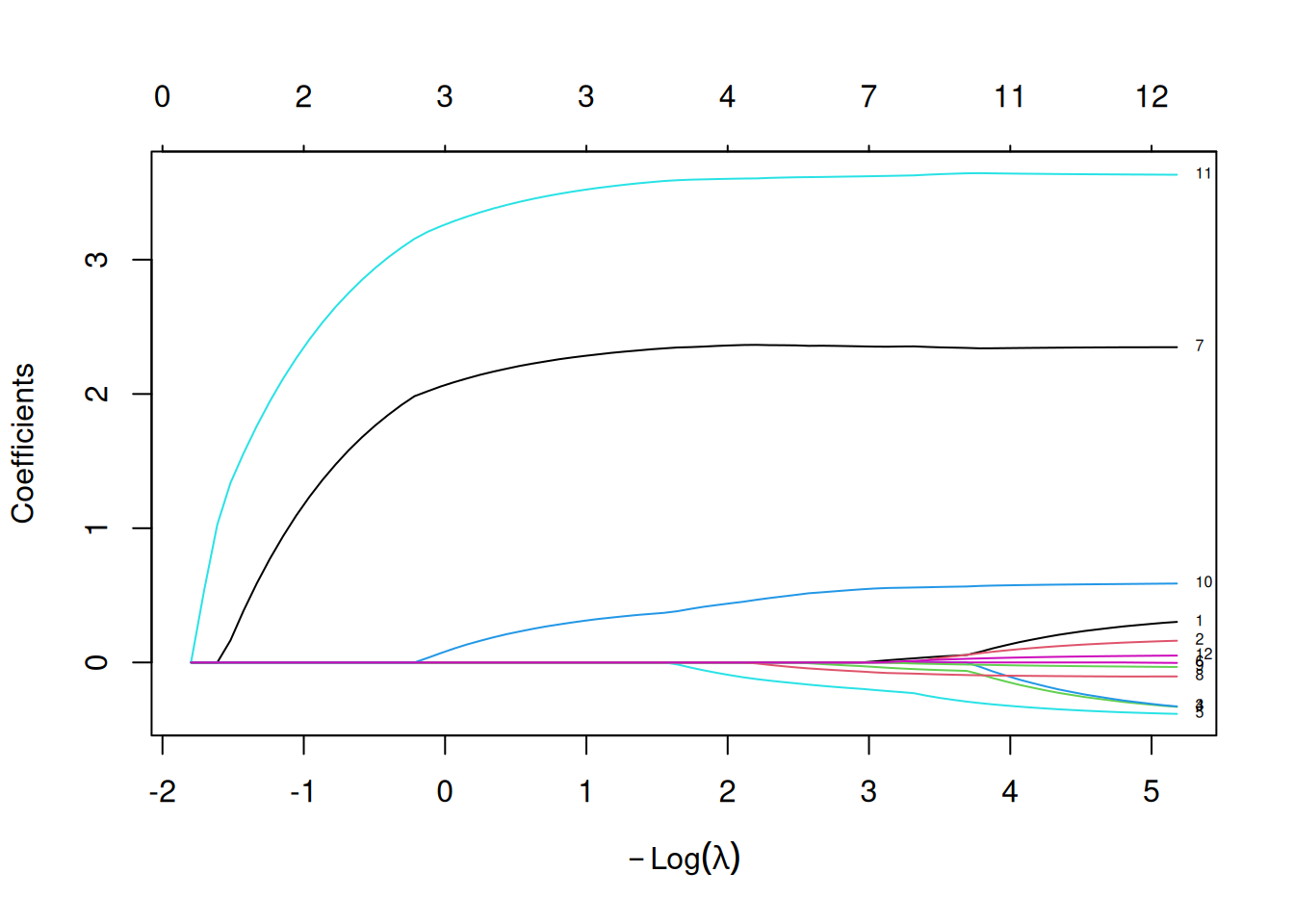
# by default this returns many Lasso models, fitted across a range of lambda values
# and we can plot a whole path of models, to see how coefficients change as a function of lambda
plot(fit, xvar="lambda", label=TRUE)

train Lasso model

# To train Lasso model we can use k-fold cross validation
# We can use cv.glmnet() function for that
# Alternatively, we could try writing our code from scratch doing more data splits...
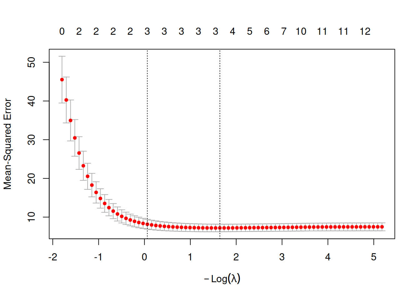
cv <- cv.glmnet(x, y, alpha = 1)

# plot MSE as a function of the lambda
plot(cv)

create final model

# `lambda.min` gives the lowest cross-validation error.
# `lambda.1se` gives a more strongly regularized, simpler model
# whose error is still within one standard error of the minimum.
# lambda.1se is often preferred when a simpler, more regularized
# model is desired with little loss in predictive performance.

cv$lambda.1se

[1] 0.9393291

# fit the final model with the selected lambda value
fit_final <- glmnet(x, y, alpha = 1, lambda =cv$lambda.1se) 

# check model coefficients. "." indicates 0
coef(fit_final)

13 x 1 sparse Matrix of class "dgCMatrix"
                    s0
(Intercept) 28.8212016
chol         .        
stab.glu     .        
hdl          .        
ratio        .        
glyhb        .        
age          .        
weight       2.0834135
bp.1s        .        
bp.1d        .        
waist        0.1062243
hip          3.2879569
time.ppn     .        

We can see that the largest coefficients (in terms of absolute values) are for weight and height, which of course it makes sense as we are predicting BMI that was defined based on weight and height in the first place. This is naturally for demonstration purposes only.

predict BMI

# Let's see how the model performs on new unseen test data
x_test <- model.matrix(BMI ~.-1, data_test)
y_pred <- fit_final %>% predict(x_test) %>% as.vector()

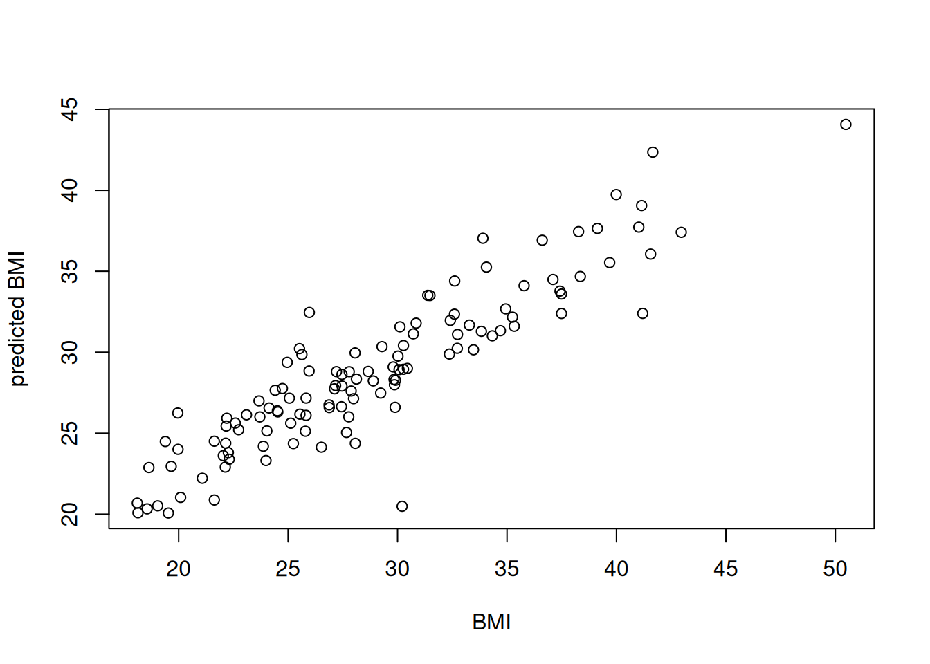
plot(data_test$BMI, y_pred, xlab = "BMI", ylab = "predicted BMI")

cor(data_test$BMI, y_pred)

[1] 0.9095373