Exercises (regression coefficients)

Exercise 1 (Dose, genotype and enzyme activity) An experiment investigates how the activity of an enzyme changes with drug dose. Measurements were obtained from two genotypes, WT and Mutant, and samples were processed in three experimental batches.

Copy and run the code below to create the data.

genotype <- factor(
  rep(c("WT", "Mutant"), each = 24),
  levels = c("WT", "Mutant")
)

dose <- rep(
  rep(c(0, 2, 4, 6, 8, 10), each = 4),
  2
)

batch <- factor(
  rep(c("B1", "B2", "B3"), length.out = 48),
  levels = c("B1", "B2", "B3")
)

activity <- c(
  13.43, 13.44, 10.60, 10.36,
  12.34, 13.12, 12.75, 13.67,
  14.61, 15.53, 13.64, 16.10,
  14.77, 20.82, 17.47, 16.79,
  21.95, 18.53, 20.10, 20.34,
  21.73, 22.38, 20.82, 19.50,
  14.65, 14.93, 10.53, 16.83,
  15.47, 13.89, 15.64, 19.03,
  22.03, 20.09, 20.89, 19.93,
  23.02, 24.61, 21.32, 24.07,
  28.11, 22.73, 26.46, 27.81,
  29.73, 28.64, 28.97, 27.76
)

enzyme <- data.frame(
  activity,
  dose,
  genotype,
  batch
)

head(enzyme)

  activity dose genotype batch
1    13.43    0       WT    B1
2    13.44    0       WT    B2
3    10.60    0       WT    B3
4    10.36    0       WT    B1
5    12.34    2       WT    B2
6    13.12    2       WT    B3

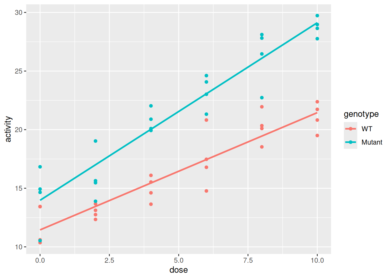
1. Make an exploratory plot of activity against dose, using different colours for the two genotypes. What patterns do you see?

2. Fit a linear model in R to model enzyme activity given dose, genotype and batch.

3. What are the reference categories for genotype and batch?

4. Given the fitted model, what is the expected enzyme activity for a Mutant sample with a dose of 5 from batch B2? Calculate using the model and check your calculations using predict() function.

5. Which model coefficients show evidence of an association with enzyme activity at the 5% significance level?

Solution

ggplot(enzyme, aes(x = dose, y = activity, colour = genotype)) +
  geom_point() +
  geom_smooth(method = "lm", se = FALSE)

`geom_smooth()` using formula = 'y ~ x'

Enzyme activity appears to increase with increasing dose. The Mutant samples also tend to have higher enzyme activity than the WT samples.

model1 <- lm(
  activity ~ dose + genotype + batch,
  data = enzyme
)

summary(model1)

Call:
lm(formula = activity ~ dose + genotype + batch, data = enzyme)

Residuals:
    Min      1Q  Median      3Q     Max 
-3.7464 -0.8783  0.1982  1.0280  3.2338 

Coefficients:
               Estimate Std. Error t value Pr(>|t|)    
(Intercept)    10.19616    0.61019  16.710  < 2e-16 ***
dose            1.27206    0.07497  16.968  < 2e-16 ***
genotypeMutant  5.09792    0.50846  10.026 7.97e-13 ***
batchB2         0.69710    0.62386   1.117    0.270    
batchB3        -1.01768    0.62722  -1.623    0.112    
---
Signif. codes:  0 '***' 0.001 '**' 0.01 '*' 0.05 '.' 0.1 ' ' 1

Residual standard error: 1.761 on 43 degrees of freedom
Multiple R-squared:  0.9015,    Adjusted R-squared:  0.8924 
F-statistic:  98.4 on 4 and 43 DF,  p-value: < 2.2e-16

The reference categories are: WT for genotype and B1 for batch.

The coefficients for genotypeMutant, batchB2 and batchB3 therefore describe differences relative to these reference categories.

From the fitted model,

\[ \widehat{activity} = 10.196 + 1.272 \cdot dose + 5.098 \cdot I_{\text{Mutant}} + 0.697 \cdot I_{\text{B2}} - 1.018 \cdot I_{\text{B3}}. \]

For a Mutant sample with dose = 5 from batch B2:

\[ \widehat{activity} = 10.196 + 1.272 \cdot 5 + 5.098 + 0.697 \approx 22.35. \]

We can also obtain the prediction in R:

new_sample <- data.frame(
  dose = 5,
  genotype = factor("Mutant", levels = levels(enzyme$genotype)),
  batch = factor("B2", levels = levels(enzyme$batch))
)

predict(model1, newdata = new_sample)

       1 
22.35146 

At the 5% significance level:

• dose shows evidence of an association with enzyme activity (\(p < 2\times10^{-16}\));
• genotypeMutant shows evidence of an association with enzyme activity (\(p = 7.97\times10^{-13}\));
• there is no evidence that batchB2 differs from the reference batch B1 (\(p = 0.270\));
• there is no evidence that batchB3 differs from the reference batch B1 (\(p = 0.112\)).

Thus, dose and genotype are clearly associated with enzyme activity in this fitted model, while the individual batch coefficients are not significantly different from the reference batch.

Exercise 2 (Treatment response) A clinical study investigates whether a biomarker and treatment are associated with the probability of responding to treatment.

The outcome response is coded as:

• 1: responded to treatment
• 0: did not respond

The data also contain:

• marker: a continuous biomarker measurement
• treatment: either Control or Drug
• age: age in years

Copy and run the code below to create the data.

response <- c(
  0,1,0,0,1,1,1,1,0,1,
  0,0,0,1,1,1,1,1,0,1,
  0,0,0,1,0,1,1,1,0,1,
  0,0,0,1,0,1,1,1,1,1,
  1,1,1,1,0,1,0,1,0,1,
  0,0,0,0,0,1,1,1,0,1
)

marker <- rep(
  c(0.5, 1, 1.5, 2, 2.5, 3, 3.5, 4, 1.2, 2.8),
  6
)

treatment <- factor(
  rep(c("Control", "Drug"), 30),
  levels = c("Control", "Drug")
)

age <- rep(
  c(35, 42, 51, 60, 67, 48, 55, 39, 63, 45),
  6
)

trial <- data.frame(
  response,
  marker,
  treatment,
  age
)

head(trial)

  response marker treatment age
1        0    0.5   Control  35
2        1    1.0      Drug  42
3        0    1.5   Control  51
4        0    2.0      Drug  60
5        1    2.5   Control  67
6        1    3.0      Drug  48

1. Fit a logistic regression model to model the probability of response given marker, treatment and age.

2. What is the reference category for treatment? What comparison does the coefficient treatmentDrug therefore represent?

3. Using the Wald tests reported in the model summary, which coefficients show evidence of an association with the probability of response at the 5% significance level?

4. The estimated coefficient for marker is approximately \(1.75\).

• Calculate the corresponding odds ratio.
• Interpret this odds ratio in the context of the study.

5. The estimated coefficient for treatmentDrug is approximately \(1.51\).

• Calculate the corresponding odds ratio.
• Interpret this odds ratio in the context of the study.

6. Using the fitted model, estimate the probability of response for a 50-year-old patient with a marker value of 2.5 who receives the Drug treatment. Check your answer using predict() with type = "response".

Solution

Fit the logistic regression model:

model2 <- glm(
  response ~ marker + treatment + age,
  family = binomial(link = "logit"),
  data = trial
)

summary(model2)

Call:
glm(formula = response ~ marker + treatment + age, family = binomial(link = "logit"), 
    data = trial)

Coefficients:
              Estimate Std. Error z value Pr(>|z|)    
(Intercept)   -0.96994    2.18446  -0.444 0.657031    
marker         1.75274    0.51477   3.405 0.000662 ***
treatmentDrug  1.50666    0.76777   1.962 0.049717 *  
age           -0.05776    0.04477  -1.290 0.197067    
---
Signif. codes:  0 '***' 0.001 '**' 0.01 '*' 0.05 '.' 0.1 ' ' 1

(Dispersion parameter for binomial family taken to be 1)

    Null deviance: 82.108  on 59  degrees of freedom
Residual deviance: 47.317  on 56  degrees of freedom
AIC: 55.317

Number of Fisher Scoring iterations: 6

The reference category for treatment is Control.

Therefore, the coefficient treatmentDrug compares patients receiving the Drug treatment with patients receiving the Control treatment, while marker and age are held constant.

At the 5% significance level:

• marker shows evidence of an association with the probability of response (\(p = 0.000662\));
• treatmentDrug shows evidence of an association with the probability of response (\(p = 0.0497\));
• age does not show evidence of an association with the probability of response (\(p = 0.197\)).

4. The estimated coefficient for marker is

\[ \hat{\beta}_{marker} = 1.753. \]

The corresponding odds ratio is

\[ \exp(1.753) \approx 5.77. \]

Thus, for a one-unit increase in marker, the odds of treatment response are estimated to be approximately 5.8 times higher, with treatment and age held constant.

5. The estimated coefficient for treatmentDrug is

\[ \hat{\beta}_{Drug} = 1.507. \]

The corresponding odds ratio is

\[ \exp(1.507) \approx 4.51. \]

Thus, patients receiving the Drug have approximately 4.5 times the odds of response compared with patients receiving Control, with marker and age held constant.

The odds ratios can also be calculated in R:

#|code-fold: false
exp(coef(model2))

  (Intercept)        marker treatmentDrug           age 
    0.3791070     5.7703864     4.5116284     0.9438804 

For a 50-year-old patient with marker = 2.5 receiving the Drug, the fitted log-odds are

\[ -0.970 + 1.753(2.5) + 1.507 - 0.058(50) \approx 2.03. \]

Converting the log-odds to a probability gives

\[ p = \frac{\exp(2.03)} {1+\exp(2.03)} \approx 0.884. \]

Thus, the fitted model predicts a probability of response of approximately 88%.

We can check this directly in R:

new_patient <- data.frame(
  marker = 2.5,
  treatment = factor(
    "Drug",
    levels = levels(trial$treatment)
  ),
  age = 50
)

predict(
  model2,
  newdata = new_patient,
  type = "response"
)

        1 
0.8839909