4 Repeating the sampling
Statistical Methods for Life Sciences
4.1 From individual observations to study results
So far, we have used probability models to describe the height of one randomly selected student.
In a study, however, we usually observe several individuals and calculate a summary, such as the sample mean.
If we repeated the study with different students, would we obtain the same sample mean?
A parameter describes a population. For example, the population mean height is denoted by \(\mu\).
A statistic is calculated from a sample. For example, the sample mean is
\[ \bar{X}=\frac{1}{n}\sum_{i=1}^{n}X_i. \]
Before collecting the data, \(\bar{X}\) is a random variable because its value depends on which individuals are selected.
After collecting the data, we obtain one observed value, denoted by \(\bar{x}\).
4.2 Imagine repeating the study
Consider our hypothetical population of student heights, with
\[ \mu=170\text{ cm} \qquad\text{and}\qquad \sigma=7\text{ cm}. \]
Imagine repeating the following study many times:
- Randomly select five students.
- Measure their heights.
- Calculate their mean height.
- Record the mean and select a new sample.
Each sample is likely to contain different students, so the sample means will not all be identical.
Provided that the observations are sampled independently from the same population, the expected value of the sample mean is the population mean:
\[ E[\bar{X}]=\mu=170\text{ cm}. \]
The distribution of the sample means across repeated studies is called the sampling distribution of the sample mean.
Note
The population distribution describes variation among individuals.
The sampling distribution describes variation among statistics calculated from different samples.
4.3 Simulating repeated studies
We can explore the sampling distribution by simulating many independent studies from our normal population model.
Before looking at the results, predict:
- Will sample means vary as much as individual heights?
- What will happen if each study includes 100 students rather than five?
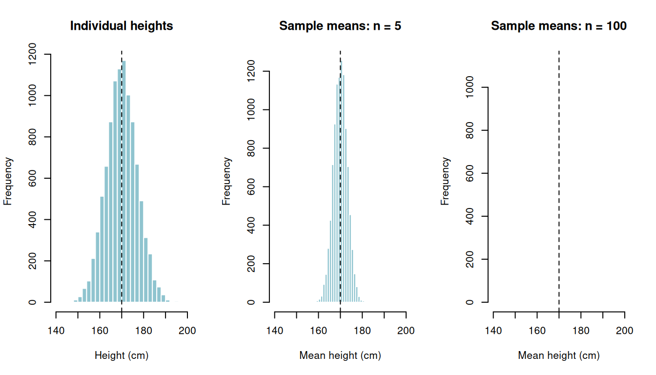
All three distributions are centred near the population mean of 170 cm.
However:
- Individual heights show substantial variation.
- Means based on five students vary less than individual heights.
- Means based on 100 students vary much less.
Thus, sample means vary less than individual observations, and means based on larger samples vary less than means based on smaller samples.
This principle is not limited to means. Other statistics, such as a sample proportion or a difference between two means, also have sampling distributions.
4.4 Why do the sample means look normal?
In this example, individual heights follow a normal distribution. The mean of independent observations from a normal population is therefore also normally distributed.
The central limit theorem extends this result beyond normal populations:
For many population distributions, the sampling distribution of the sample mean becomes approximately normal as the sample size increases.
This does not mean that the individual observations become normally distributed. It is the distribution of the sample mean across repeated samples that becomes approximately normal.
How large the sample must be for a useful approximation depends on the shape of the population distribution and the presence of extreme values.
4.5 What if we have only one study?
The previous simulation assumes that we know the population model and can generate many new samples from it.
In practice, we usually have only one observed sample.
For example, if we measure 20 students, we have one sample containing 20 observations—not 20 independent samples.
Can we use this sample to approximate how the sample mean might vary across repeated studies?
4.5.1 Bootstrap: resampling the observed data
The bootstrap treats the observed sample as an approximation of the population and repeatedly resamples from it.
Imagine writing the 20 observed heights on cards:
- Draw one card at random, record its value and return it.
- Repeat until 20 values have been drawn.
- Calculate their mean.
- Repeat the procedure many times.
The cards are returned after every draw, so sampling is performed with replacement. An observed height can therefore appear more than once in a bootstrap sample, while another may not appear at all.
Sampling without replacement would not work: selecting all 20 cards would reproduce the original sample and therefore always give the same mean.
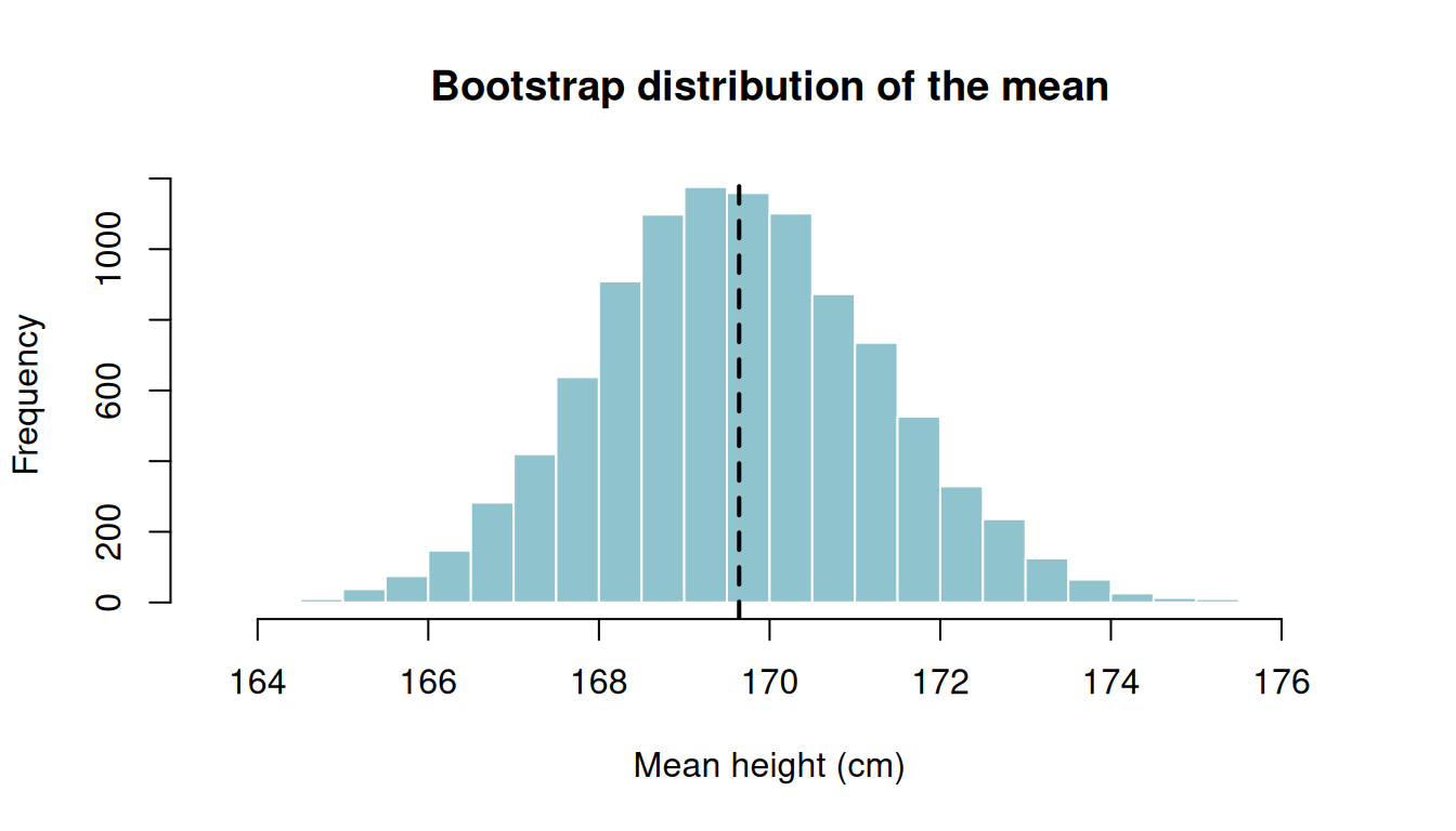
The bootstrap means are centred near the observed sample mean, not necessarily the true population mean.
The spread of the bootstrap distribution approximates how much the sample mean would vary across repeated samples.
Bootstrapping does not create new biological information. Its results still depend on whether the original sample adequately represents the population.
This simple bootstrap also assumes independent observations. It cannot correct selection bias or compensate for a poorly designed study.
Key message
A statistic, such as a sample mean, varies from sample to sample.
The distribution of its possible values across repeated samples is called its sampling distribution.
Sample means vary less than individual observations, and means based on larger samples generally vary less.
Next, we need a way to quantify the spread of the sampling distribution. This leads to the standard error.