6 Exercises

Statistical Methods for Life Sciences

Exercises

Exercise 6.1 (What is random?) We randomly select 10 adults from a defined population and record their BMI. The first person’s BMI is 24.5.

Let’s model as BMI as a continuous, positive measurement.

Identify:

The sample size.
The sample space for one BMI measurement.
The random variable.
Its observed value.
An example event involving BMI.

Solution

Sample size: \(n = 10\).
Sample space: \(S = [0, \infty)\) under our positive, continuous model.
Random variable: \(X =\) the BMI of the first randomly selected adult.
Observed value: \(x = 24.5\).
Example event: the first adult’s BMI exceeds 25, \(E = \{X > 25\}\).

Exercise 6.2 (What can we calculate — and what is missing?) Suppose 50% of adults in our hypothetical population have a BMI above 25.

For an adult randomly selected from this population:

What is the probability that their BMI is 25 or less?
Can we calculate the probability that their BMI exceeds 30 from this information alone?

Solution

By the complement rule:

\[ P(X\leq25)=1-P(X>25)=1-0.50=0.50. \]

We cannot calculate \(P(X>30)\) exactly from this information.

Because \(\{X>30\}\subseteq\{X>25\}\), we know only that:

\[ 0\leq P(X>30)\leq0.50. \]

Exercise 6.3 (A probability model for BMI) In the previous exercise, knowing only that 50% of adults have a BMI above 25 was not enough to calculate the probability of a BMI above 30.

Suppose we now use the following probability model for BMI in our hypothetical population:

\[ X \sim N(25,4^2). \]

For one randomly selected adult, calculate in R:

What is the probability that their BMI exceeds 30?
What is the probability that their BMI is between 20 and 30?
How many standard deviations above the mean is a BMI of 30?
Below which BMI value do 95% of adults fall according to this model?

Solution

The model tells us that

\[ \mu=25, \qquad \sigma=4. \]

For a BMI above 30:

\[ P(X>30)=1-F(30). \]

In R:

pnorm(30, mean = 25, sd = 4, lower.tail = FALSE)

[1] 0.1056498

For a BMI between 20 and 30:

\[ P(20<X<30)=F(30)-F(20). \]

pnorm(30, mean = 25, sd = 4) -
  pnorm(20, mean = 25, sd = 4)

[1] 0.7887005

To locate a BMI of 30 relative to the mean, we standardise:

\[ z = \frac{30-25}{4} = 1.25. \]

A BMI of 30 is therefore 1.25 standard deviations above the mean.

We can also calculate the upper-tail probability using the standard normal distribution:

z <- (30 - 25) / 4

pnorm(z, lower.tail = FALSE)

[1] 0.1056498

For the 95th percentile, we want the value \(x_{0.95}\) such that

\[ P(X \leq x_{0.95}) = 0.95. \]

On the standard normal scale,

\[ z_{0.95} = \Phi^{-1}(0.95) \approx 1.645. \]

In R:

qnorm(0.95)

[1] 1.644854

We then transform back to the BMI scale:

\[ x_{0.95} = \mu+\sigma z_{0.95} = 25+4(1.645) \approx31.6. \]

So approximately 95% of adults have a BMI below 31.6 under this model.

We can also calculate the cutoff directly in R:

qnorm(0.95, mean = 25, sd = 4)

[1] 31.57941

Exercise 6.4 (A discrete probability model) Suppose that 15% of bacterial isolates from a particular population are resistant to an antibiotic.

We randomly and independently select 30 isolates and let \(K\) be the number that are resistant.

What distribution is appropriate for \(K\)? Specify its parameters.
What values can \(K\) take?
What is the expected number of resistant isolates?
What is the probability that exactly 4 isolates are resistant?
What is the probability that 4 or more isolates are resistant?
Simulate 10,000 values of \(K\) in R. Use the simulated values to approximate the probability that 4 or more isolates are resistant. Compare your estimate with the exact probability calculated above.

Solution

For each isolate, resistance is a binary outcome:

\[ Y = \begin{cases} 1, & \text{resistant},\\ 0, & \text{not resistant}. \end{cases} \]

with

\[ P(Y=1)=p=0.15. \]

Thus,

\[ Y \sim \operatorname{Bernoulli}(0.15). \] The number of resistant isolates among 30 independent isolates is

\[ K=\sum_{i=1}^{30}Y_i, \]

\[ K\sim\operatorname{Bin}(30,0.15). \]

The possible values are

\[ K\in\{0,1,2,\ldots,30\}. \] c)

The expected number of resistant isolates is

\[ E[K] = np = 30\times0.15 = 4.5. \]

For exactly four resistant isolates,

\[ P(K=4) = \binom{30}{4} (0.15)^4(0.85)^{26}. \]

In R:

dbinom(4, size = 30, prob = 0.15)

[1] 0.2028089

For four or more resistant isolates,

\[ P(K\geq4) = 1-P(K\leq3). \]

In R:

1 - pbinom(3, size = 30, prob = 0.15, lower.tail = TRUE)

[1] 0.6783401

# or
pbinom(3, size = 30, prob = 0.15, lower.tail = FALSE)

[1] 0.6783401

We can simulate repeated samples from the binomial model:

set.seed(2026)

K_sim <- rbinom(
  10000,
  size = 30,
  prob = 0.15
)

The simulated probability of observing four or more resistant isolates is:

mean(K_sim >= 4)

[1] 0.6756

This should be close to the exact probability obtained above:

pbinom(
  3,
  size = 30,
  prob = 0.15,
  lower.tail = FALSE
)

[1] 0.6783401

We can simulate repeated samples from the binomial model:

set.seed(2026)

K_sim <- rbinom(
  10000,
  size = 30,
  prob = 0.15
)

The simulated probability of observing four or more resistant isolates is:

mean(K_sim >= 4)

[1] 0.6756

This should be close to the exact probability:

pbinom(
  3,
  size = 30,
  prob = 0.15,
  lower.tail = FALSE
)

[1] 0.6783401

The simulated value will not be exactly the same because it is based on a finite number of random simulations. With many simulations, the estimate tends to get closer to the model probability.

Exercise 6.5 (How precise is the estimated mean?) A random sample of 36 adults has

\[ \bar{x}=26.2 \]

and sample standard deviation

\[ s=3.6. \]

Suppose we want to compare the observed mean BMI with a value of 25.

Estimate the standard error of the sample mean.
How far is the observed sample mean from 25, measured in estimated standard error units?
Should we compare this standardised statistic with a standard normal distribution or a t-distribution? Why?
How many degrees of freedom does the t-distribution have?
If we instead sampled 100 adults and obtained approximately the same sample SD, what would happen to the standard error?

Solution

Because the population SD, \(\sigma\), is unknown, we estimate the standard error using the sample SD:

\[ \widehat{\operatorname{SE}}(\bar X) = \frac{s}{\sqrt n}. \]

For \(n=36\) and \(s=3.6\),

\[ \widehat{\operatorname{SE}}(\bar X) = \frac{3.6}{\sqrt{36}} = \frac{3.6}{6} = 0.6. \]

The observed mean is

\[ 26.2-25=1.2 \]

BMI units above 25.

In estimated standard error units,

\[ T = \frac{\bar{x}-25} {s/\sqrt n} = \frac{26.2-25}{0.6} = 2. \]

So the observed mean is 2 estimated standard errors above 25.

Because \(\sigma\) is unknown and has been replaced by the sample SD, \(s\), the appropriate reference distribution is a t-distribution.

For a one-sample mean,

\[ df=n-1=35. \]

Therefore,

\[ T\sim t_{35} \]

under the corresponding normal population model.

If \(n=100\) and \(s\approx3.6\),

\[ \widehat{\operatorname{SE}}(\bar X) = \frac{3.6}{\sqrt{100}} = 0.36. \]

The larger sample therefore gives a smaller standard error and a more precise estimate of the population mean.

Exercise 6.6 (Estimating uncertainty with the bootstrap) Suppose we observe BMI in a sample of 20 adults:

bmi <- c(
  21.8, 22.4, 23.1, 23.7, 24.0,
  24.3, 24.8, 25.0, 25.2, 25.5,
  25.9, 26.1, 26.4, 26.8, 27.1,
  27.5, 28.0, 28.6, 29.2, 30.1
)

Calculate the observed sample mean.
Create one bootstrap sample by sampling 20 observations from bmi with replacement. Calculate its mean.
Repeat this procedure 5,000 times and store the bootstrap means.
Plot the distribution of the bootstrap means. Around what value is the bootstrap distribution centred?
Use the bootstrap distribution to estimate the probability that a bootstrap sample mean is greater than 26.
Use the bootstrap distribution to estimate the standard error of the sample mean.
Compare the bootstrap estimate of SE with the usual estimate: \(\frac{s}{\sqrt{n}}\)

Solution

The observed sample mean is:

mean(bmi)

[1] 25.775

A single bootstrap sample is obtained by sampling from the observed values with replacement:

set.seed(2026)

bmi_boot <- sample(
  bmi,
  size = length(bmi),
  replace = TRUE
)

mean(bmi_boot)

[1] 25.66

The bootstrap sample contains the same number of observations as the original sample, but some observations may appear more than once and others may not appear at all.

We repeat the resampling procedure many times:

set.seed(2026)

bootstrap_means <- replicate(
  5000,
  mean(
    sample(
      bmi,
      size = length(bmi),
      replace = TRUE
    )
  )
)

Each value in bootstrap_means is the mean of one bootstrap sample.

We can inspect the empirical distribution of the bootstrap means:

hist(
  bootstrap_means,
  breaks = 30,
  main = "",
  xlab = "Bootstrap mean BMI"
)

abline(
  v = mean(bmi),
  lty = 2,
  lwd = 2
)

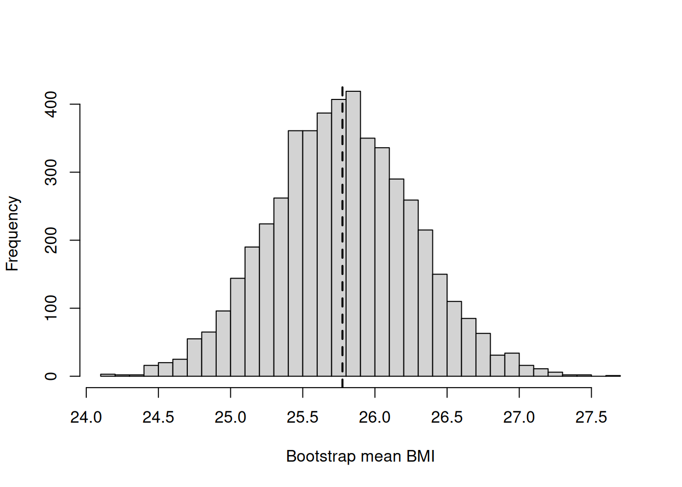
The bootstrap distribution should be centred close to the observed sample mean.

We can estimate the probability that a bootstrap sample mean exceeds 26 by calculating the proportion of bootstrap means above 26:

mean(bootstrap_means > 26)

[1] 0.3222

This estimates

\[ P(\bar{X}^*>26), \]

where \(\bar{X}^*\) denotes a bootstrap sample mean.

The bootstrap estimate of the standard error is the standard deviation of the bootstrap means:

sd(bootstrap_means)

[1] 0.4961505

Thus,

\[ \widehat{\operatorname{SE}}_{\text{bootstrap}} = \operatorname{SD}(\bar{X}^*). \]

The usual estimated standard error of the sample mean is

\[ \widehat{\operatorname{SE}}(\bar X) = \frac{s}{\sqrt n}. \]

In R:

sd(bmi) / sqrt(length(bmi))

[1] 0.5015699

The two estimates should be similar.

The bootstrap uses repeated resampling of the observed data to construct an empirical distribution of the statistic. This distribution can be used to study its variability and, when appropriate, estimate probabilities under the resampling scheme.