Variant filtering

Author

Per Unneberg

Published

15-Nov-2023

Compute environment setup

If you haven’t already done so, please read Compute environment for information on how to prepare your working directory.

In this exercise we will look at ways of filtering variant data. We will begin by applying filters to the variant file containing variant sites only, followed by an approach that filters on sequencing depth in a variant file containing both variant and invariant sites. The latter methodology can then be generalized to generate depth-based filters from BAM files.

Important

The commands of this document have been run on a subset (a subregion) of the data. Therefore, although you will use the same commands, your results will differ from those presented here.

Learning objectives

filter variants by quality, read depth, and other metrics
apply filters to a VCF file
create per sample, per population, and total depth of coverage profiles
generate mask files for downstream processing

Data setup

UPPMAX
Local

Move to your course working directory /proj/naiss2023-22-1084/users/USERNAME, create an exercise directory called monkeyflower and cd to it:

cd /proj/naiss2023-22-1084/users/USERNAME
mkdir -p monkeyflower
cd monkeyflower

Retrieve the data with rsync. You can use the --dry-run option to see what is going to happen; just remove it when you are content:

rsync --dry-run -av \
      /proj/naiss2023-22-1084/webexport/monkeyflower/LG4/* .
# Remove the dry run option to actually retrieve data. The dot is
# important!
rsync -av /proj/naiss2023-22-1084/webexport/monkeyflower/LG4/* .

Create an exercise directory called monkeyflower and cd to it:

mkdir -p monkeyflower
cd monkeyflower

Retrieve the variant files from https://export.uppmax.uu.se/naiss2023-22-1084/monkeyflower/LG4 with wget¹:

wget --user pgip --password PASSWORD \
     --recursive --accept='*.*' \
     --reject='*.gif','index*' \
     --no-parent --no-directories \
     --no-clobber \
     --directory-prefix=. \
     https://export.uppmax.uu.se/naiss2023-22-1084/monkeyflower/LG4/

Tools

bcftools (Danecek et al., 2021)
bedtools (Quinlan & Hall, 2010)
csvtk
mosdepth (Pedersen & Quinlan, 2018)
seqkit (Shen et al., 2016)
vcflib (Garrison et al., 2022)
vcftools (Danecek et al., 2011)

Execute the following command to load modules:

module load uppmax bioinfo-tools \
    mosdepth/0.3.3 BEDTools/2.29.2 \
    samtools/1.17 bcftools/1.17 \
    vcftools/0.1.16 vcflib/1.0.1

csvtk has been manually added to the module system and can be loaded as follows:

module use /proj/naiss2023-22-1084/modules
module load csvtk

Copy the contents to a file environment.yml and install packages with mamba env update -f environment.yml.

channels:
  - conda-forge
  - bioconda
  - default
dependencies:
  - bedtools=2.31.0
  - bcftools=1.15.1
  - csvtk=0.28.0
  - mosdepth=0.3.3
  - samtools=1.15.1
  - vcflib=1.0.1
  - vcftools=0.1.16

Background

Regardless of how a raw variant call set has been produced, the calls will be of varying quality for a number of reasons. For high-coverage sequencing, the two most common are incompleteness of the reference sequence and misalignments in repetitive regions (Li, 2014). Low-coverage sequencing comes with its own biases and issues, with the most important being the difficulty to accurately call genotypes (Maruki & Lynch, 2017).

In order to improve the accuracy of downstream inference, a number of analysis-dependent quality control filters should be applied to the raw variant call set (for a concise summary, see Lou et al. (2021)). In this exercise, we will begin by applying filters to the variant file containing variant sites only, followed by a more general approach based on depth filtering of a variant file consisting of all sites, variant as well as invariant. If time permits, we will also look at an approach that generates depth profiles directly from read mappings (BAM files) and that works also when it is impractical due to file size to include invariant sites in the variant file.

It is worthwhile to spend time thinking about filtering. As we will see, there are numerous metrics to filter on, and different applications require different filters. This is not as straightforward as it first may seem, and even experts struggle to get filtering settings right.

Some recommended data filters

There are many ways to filter data. Choosing the right set of filters is not easy, and choosing appropriate thresholds depends on application, among other things. Below we list some recommended data filters and thresholds that have general applicability and recently have been reviewed (Lou et al., 2021, Table 3):

depth: Given the difficulty of accurately genotyping low-coverage sites, it is recommended to set a minimum read depth cutoff to remove false positive calls. It is also recommended to set a maximum depth cutoff as excessive coverage is often due to mappings to repetitive regions. The thresholds will depend on the depth profile over all sites, but is usually chosen as a range around the mean or median depth (e.g. lower threshold 0.8X mean, upper threshold median + 2 standard deviations).
minimum number of individuals: To avoid sites with too much missing data across individuals, a common requirement is that a minimum number (fraction) of individuals, say 75%, have sequence coverage (depth-based filter) or genotype calls.
quality (p-value): Most variant calling software provide a Phred-scaled probability score that a genotype is a true genotype. Quality values below 20 (i.e., 1%) should not be trusted, but could be set much higher (i.e., lower p-value) depending on application. Note that if a VCF file includes invariant sites, they have quality values set to 0, which renders quality based filtering inappropriate.
MAF: Filter sites based on a minimum minor allele frequency (MAF) threshold. The appropriate choice depends on application. For instance, for PCA or admixture analyses, low-frequency SNPs are uninformative, and a reasonably large cutoff (say, 0.05-0.10) could be set. If an analysis depends on invariant sites, this filter should not be applied.

Important

For applications where invariant sites should be included, such as genetic diversity calculations, neither quality nor MAF filtering should be applied.

Basic filtering of a VCF file²

We will begin by creating filters for a VCF file consisting of variant sites only for red and yellow ecotypes. Before we start, let’s review some statistics for the entire (unfiltered) call set:

bcftools stats variantsites.vcf.gz | grep ^SN

SN  0   number of samples:  10
SN  0   number of records:  128395
SN  0   number of no-ALTs:  0
SN  0   number of SNPs: 105508
SN  0   number of MNPs: 0
SN  0   number of indels:   23086
SN  0   number of others:   0
SN  0   number of multiallelic sites:   10412
SN  0   number of multiallelic SNP sites:   2108

Keep track of these numbers as we will use them to evaluate the effects of filtering.

Generate random subset of variants

Depending on the size of a study, both in terms of reference sequence and number of samples, the VCF output can become large; a VCF file may in fact contain millions of variants and be several hundred GB! We want to create filters by examining distributions of VCF quality metrics and setting reasonable cutoffs. In order to decrease run time, we will look at a random sample of sites. We use the vcflib program vcfrandomsample to randomly sample approximately 100,000 sites from our VCF file³:

# Set parameter r = 100000 / total number of variants
bcftools view variantsites.vcf.gz | vcfrandomsample -r 0.8 |\
    bgzip -c > variantsites.subset.vcf.gz
bcftools index variantsites.subset.vcf.gz
bcftools stats variantsites.subset.vcf.gz |\
    grep "number of records:"

SN  0   number of records:  103044

The -r parameter sets the rate of sampling which is why we get approximately 100,000 sites. You will need to adjust this parameter accordingly.

We will now use vcftools to compile statistics. By default, vcftools outputs results to files with a prefix out. in the current directory. You can read up on settings and options by consulting the man pages with man vcftools⁴. Therefore, we define a variable OUT where we will output our quality metrics, along with a variable referencing our variant subset:

mkdir -p vcftools
OUT=vcftools/variantsites.subset
VCF=variantsites.subset.vcf.gz

Generate statistics for filters

vcftools can compile many different kinds of statistics. Below we will focus on the ones relevant to our data filters. We will generate metrics and plot results as we go along, with the goal of generating a set of filtering thresholds to apply to the data.

Total depth per site

To get a general overview of depth of coverage, we first generate the average depth per sample⁵:

vcftools --gzvcf $VCF --depth --out $OUT 2>/dev/null
cat ${OUT}.idepth
csvtk summary -t -f MEAN_DEPTH:mean ${OUT}.idepth

INDV    N_SITES MEAN_DEPTH
PUN-R-ELF   102847  8.56957
PUN-R-JMC   102833  9.54936
PUN-R-LH    102876  9.24544
PUN-R-MT    102826  9.44265
PUN-R-UCSD  102917  8.94361
PUN-Y-BCRD  102839  9.92774
PUN-Y-INJ   102808  8.26867
PUN-Y-LO    102807  7.82653
PUN-Y-PCT   102798  9.18246
PUN-Y-POTR  102774  8.50441
MEAN_DEPTH:mean
8.95

The average coverage over all samples is 8.9X. This actually is in the low range for a protocol based on explicitly calling genotypes. At 5X coverage, there may be a high probability that only one of the alleles has been sampled (Nielsen et al., 2011), whereby sequencing errors may be mistaken for true variation.

Then we calculate depth per site to see if we can identify reasonable depth cutoffs:

vcftools --gzvcf $VCF --site-depth --out $OUT 2>/dev/null
head -n 3 ${OUT}.ldepth

CHROM   POS SUM_DEPTH   SUMSQ_DEPTH
LG4 2130    11  21
LG4 2139    12  26

So, for each position, we have a value (column SUM_DEPTH) for the total depth across all samples.

We plot the distribution of total depths by counting how many times each depth is observed. This can be done with csvtk summary where we count positions and group (-g) by the SUM_DEPTH value:⁶

csvtk summary -t -g SUM_DEPTH -f POS:count -w 0 ${OUT}.ldepth |\
 csvtk sort -t -k 1:n |\
 csvtk plot line -t - -x SUM_DEPTH -y POS:count \
    --point-size 0.01 --xlab "Depth of coverage (X)" \
    --ylab "Genome coverage (bp)" \
    --width 9.0 --height 3.5 > $OUT.ldepth.png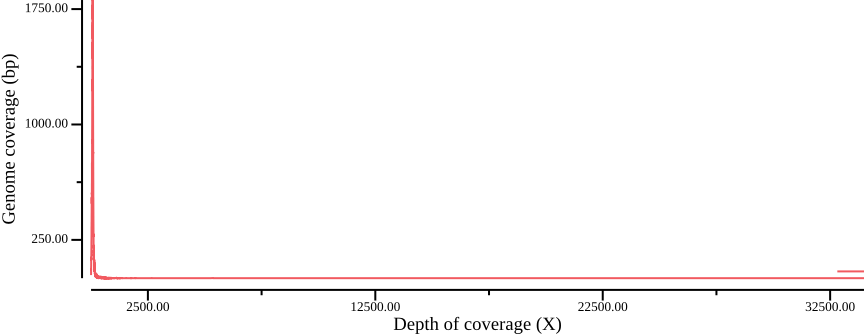

Figure 1: Distribution of the total depth per site for all samples.

On csvtk as plotting software

You are of course perfectly welcome to use R or some other software to make these plots. We choose to generate the plots using csvtk to avoid too much context switching, and also because it emulates much of the functionality in R, albeit much less powerful when it comes to plotting.

As Figure 1 shows, most sites fall within a peak, but also that there are sites with very high coverage, up to ten times as high as the depth at the peak maximum. We calculate some range statistics to get an idea of the spread. The following csvtk command will calculate the minimum, first quartile, median, mean, third quartile, and maximum of the third column (SUM_DEPTH):

csvtk summary -t -f 3:min,3:q1,3:median,3:mean,3:q3,3:max,3:stdev vcftools/variantsites.subset.ldepth

SUM_DEPTH:min   SUM_DEPTH:q1    SUM_DEPTH:median    SUM_DEPTH:mean  SUM_DEPTH:q3    SUM_DEPTH:max   SUM_DEPTH:stdev
1.00    55.00   72.00   89.28   88.00   33988.00    245.06

The range from the first quartile (q1) to the third (q3) is 55-88, showing most sites have a depth between 50-100X. We redraw the plot to zoom in on the peak:

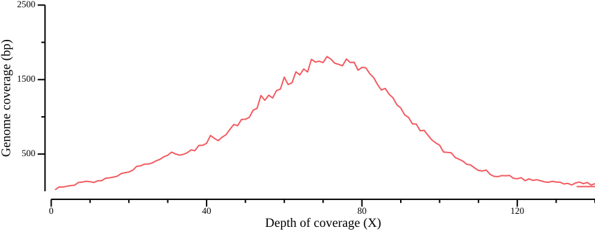
Figure 2: Zoomed in version of Figure 1 which was achieved by adding the options `--x-min 0 --x-max 140 --y-max 2500` to the plotting call.

We could choose a filter based on the quantile statistics above, or by eye-balling the graph. In this example, we could have chosen the range 50-150X, which equates to 5-15X depth per sample; note that your values will probably be different.

As an aside, we mention that there is a command to directly get the per-site mean depth, --site-mean-depth:

vcftools --gzvcf $VCF --site-mean-depth --out $OUT 2>/dev/null
head -n 3 ${OUT}.ldepth.mean

CHROM   POS MEAN_DEPTH  VAR_DEPTH
LG4 2130    1.1 0.988889
LG4 2139    1.2 1.28889

Variant quality distribution

Another quantity of interest is the variant quality. Recall, variant quality scores are Phred-scaled scores, meaning a value of 10 has a 10% chance of being wrong, 20 a 1% chance, and so on; you typically want to at least filter on 20 or even higher. We extract and plot the quality values below:

vcftools --gzvcf $VCF --site-quality --out $OUT

# To improve histogram, filter out extreme quality scores. You
# may have to fiddle with the exact values
csvtk filter -t -f "QUAL>0" -f "QUAL<1000" ${OUT}.lqual  | \
 csvtk summary -t -g QUAL -f POS:count -w 0 - |\
 csvtk sort -t -k 1:n |\
 csvtk plot hist -t --bins 100 - \
          --xlab "Quality value" \
    --ylab "Count" \
    --width 9.0 --height 3.5 > $OUT.lqual.png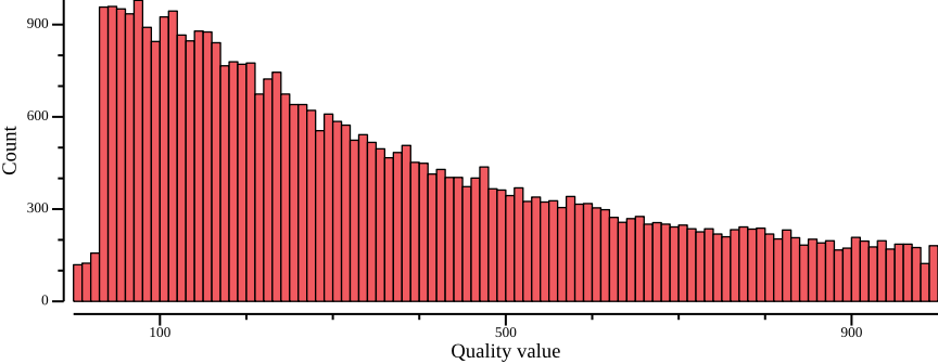

Figure 3: Distribution of variant quality scores.

Clearly most quality scores are above 20-30. For many applications, we recommend setting 30 as the cutoff.

Minor allele frequency distribution

Since we are going to calculate nucleotide diversities, we will not filter on the minor allele frequency (MAF) here. Nevertheless, we generate the distribution and plot for discussion purposes. The --freq2 will output the frequencies only, adding the option --max-alleles 2 to focus only on bi-allelic sites:

vcftools --gzvcf $VCF --freq2 --out $OUT --max-alleles 2 2>/dev/null
head -n 3 ${OUT}.frq

CHROM   POS N_ALLELES   N_CHR   {FREQ}
LG4 2130    2   14  0.857143    0.142857
LG4 2139    2   8   0.25    0.75

The last two columns are frequencies ordered according to the reference allele. Therefore, we need to pick the minimum value to get the MAF. We can use csvtk mutate to create a new column

csvtk fix -t ${OUT}.frq 2>/dev/null |\
 csvtk mutate2 -t -n maf -e '${5} > ${6} ? "${6}" : "${5}" ' - |\
 csvtk plot hist -t --bins 20 -f maf - \
       --xlab "Minor allele frequency" \
       --ylab "Count" \
       --width 9.0 --height 3.5 > $OUT.frq.png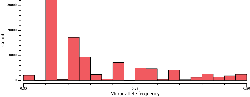

Figure 4: Distribution of minor allele frequencies.

Since our variant file consists of 10 individuals, that is, 20 chromosomes, there are only so many frequencies that we can observe, which is why the histogram looks a bit disconnected⁷. In fact, given 20 chromosomes, MAF=0.05 corresponds to one alternative allele among all individuals (singleton), MAF=0.1 to two, and so on. The maximum value is 0.5, which is to be expected, as it is a minor allele frequency. We note that there are more sites with a low minor allele frequency, which in practice means there are many singleton variants.

This is where filtering on MAF can get tricky. Singletons may correspond to sequencing error, but if too hard a filter is applied, the resulting site frequency spectrum (SFS) will be skewed. For statistics that are based on the SFS, this may lead biased estimates. Since we will be applying such a statistic, we do not filter on the MAF here. Note, however, that for other applications, such as population structure, it may be warranted to more stringently (say, MAF>0.1) filter out low-frequency variants.

Missing data for individuals and sites

The proportion missing data per individual can indicate whether the input DNA was of poor quality, and that the individual should be excluded from analysis. Note that in this case, missing data refers to a missing genotype call and not sequencing depth!

We can calculate the proportion of missing data

vcftools --gzvcf $VCF --missing-indv --out $OUT 2>/dev/null
head -n 3 ${OUT}.imiss

INDV    N_DATA  N_GENOTYPES_FILTERED    N_MISS  F_MISS
PUN-R-ELF   103044  0   6991    0.0678448
PUN-R-JMC   103044  0   6588    0.0639339

and look at the results, focusing on the F_MISS column (proportion missing sites):

csvtk plot hist -t --x-min 0 -f F_MISS ${OUT}.imiss > ${OUT}.imiss.png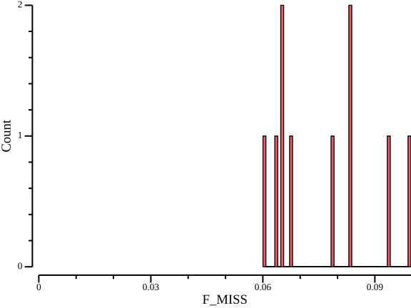

Figure 5: Distribution of missingness per sample.

Here, the proportion lies in the range 0.06-0.10 for all samples, which indicates good coverage of all samples and we refrain from taking any action.

Similarly, we can look at missingness per site. This is related to the filter based on minimum number of individuals suggested by Lou et al. (2021). We calculate

vcftools --gzvcf $VCF --missing-site --out $OUT 2>/dev/null
head -n 3 ${OUT}.lmiss

CHR POS N_DATA  N_GENOTYPE_FILTERED N_MISS  F_MISS
LG4 2130    20  0   6   0.3
LG4 2139    20  0   12  0.6

and plot to get an idea of if there are sites that lack data.

csvtk plot hist --bins 20 -t -f F_MISS ${OUT}.lmiss > ${OUT}.lmiss.png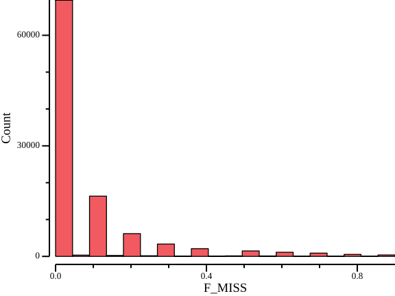

Figure 6: Distribution of missingness among sites.

As Figure 6 shows, many sites have no or little missing data, but given the low coverage, there is a non-negligible number of sites with higher missingness. We calculate range statistics to get a feeling for a good cutoff:

csvtk summary -t -f 6:min,6:q1,6:median,6:mean,6:q3,6:max vcftools/variantsites.subset.lmiss

F_MISS:min  F_MISS:q1   F_MISS:median   F_MISS:mean F_MISS:q3   F_MISS:max
0.00    0.00    0.00    0.08    0.10    0.90

The mean missingness is 8%, so we can safely use 25% missingness as threshold. Typical values of tolerated missingness lie in the range 5-25%. Note that vcftools interprets this value as 1 - missingness, so it has to be inverted to 75% when filtering!

Heterozygosity

vcftools can calculate the heterozygosity per individual. More specifically, it estimates the inbreeding coefficient F for each individual.

vcftools --gzvcf $VCF --het --out $OUT 2>/dev/null
cat ${OUT}.het

INDV    O(HOM)  E(HOM)  N_SITES F
PUN-R-ELF   72393   65584.9 87301   0.31351
PUN-R-JMC   68270   65824.3 87571   0.11246
PUN-R-LH    70890   66054.7 87882   0.22153
PUN-R-MT    69985   65776.7 87480   0.19390
PUN-R-UCSD  74700   65580.4 87550   0.41510
PUN-Y-BCRD  69345   64909.7 86275   0.20759
PUN-Y-INJ   71169   64112.6 85018   0.33754
PUN-Y-LO    72845   63349.3 84415   0.45077
PUN-Y-PCT   74452   64462.2 85937   0.46519
PUN-Y-POTR  71716   64520.3 85782   0.33844

Here, F is a measure of how much the observed homozygotes O(HOM) differ from the expected (E(HOM); expected by chance under Hardy-Weinberg equilibrium), and may be negative. vcftools calculates F from the expression $F=(O-E)/(N-E)$⁸, which you can verify by substituting the variables in the output.

If F is positive ($O(HOM) > E(HOM)$), i.e., there are more observed homozygotes than expected, then there is a deficit of heterozygotes, which could be a sign of inbreeding or signs of allelic dropout in case of low sequencing coverage.

If F is negative, there are fewer observed homozygotes than expected, or conversely, an excess of heterozygotes. This could be indicative of poor sequence quality (bad mappings) or contamination (Purcell et al., 2007).

The underlying assumption is HWE, which holds for F=0.

In this case, we know that the samples are from two different populations, red and yellow. In such cases, we actually expect a deficit of heterozygotes (and consequently, positive F) simply due to something called the Wahlund effect.

Warning

The inbreeding coefficient is a population-level statistic and is not reliable for small sample sizes ($n<10$, say). Therefore, our sample size is in the lower range and the results should be taken with a grain of salt.

Exercise

Use bcftools view -s SAMPLENAMES | vcftools --vcf - --het --stdout to calculate the heterozygosity for red and yellow samples. Substitute SAMPLENAMES for a comma-separated list of samples.

Answer

bcftools view -s PUN-R-ELF,PUN-R-JMC,PUN-R-LH,PUN-R-MT,PUN-R-UCSD $VCF |\
 vcftools --vcf - --het --stdout 2>/dev/null

INDV    O(HOM)  E(HOM)  N_SITES F
PUN-R-ELF   41624   37668.8 56532   0.20968
PUN-R-JMC   37396   37778.7 56697   -0.02023
PUN-R-LH    39806   37867.3 56798   0.10241
PUN-R-MT    38885   37615.4 56380   0.06766
PUN-R-UCSD  43543   37476.1 56393   0.32071

Filtering the VCF

Now that we have decided on filters we can apply them to the VCF. We first set the filters as variables:

MISS=0.75
QUAL=30
MIN_DEPTH=5
MAX_DEPTH=15

and run vcftools as follows:

OUTVCF=${VCF%.subset.vcf.gz}.filtered.vcf.gz
vcftools --gzvcf $VCF \
   --remove-indels --max-missing $MISS \
   --min-meanDP $MIN_DEPTH --max-meanDP $MAX_DEPTH \
   --minDP $MIN_DEPTH --maxDP $MAX_DEPTH --recode \
   --stdout 2>/dev/null |
 gzip -c > $OUTVCF

Compare the results with the original input:

bcftools stats $OUTVCF | grep "^SN"

SN  0   number of samples:  10
SN  0   number of records:  37697
SN  0   number of no-ALTs:  0
SN  0   number of SNPs: 37486
SN  0   number of MNPs: 0
SN  0   number of indels:   0
SN  0   number of others:   0
SN  0   number of multiallelic sites:   1666
SN  0   number of multiallelic SNP sites:   688

Quite a substantial portion variants have in fact been removed, which here can most likely be attributed to the low average sequencing coverage.

Depth filtering of VCF with invariant sites

Now we turn our attention to a VCF file containing variant and invariant sites. We will generate depth-based filters, with the motivation that they represent portions of the genome that are accessible to analysis, regardless of whether they contain variants or not. In so doing, we treat filtered sites as missing data and do not assume that they are invariant, as many software packages do.

Figure 7: Coverage distributions for three hypothetical samples along with the cumulative coverage for all samples.

Figure 7 illustrates the sequencing coverage of three samples. The important thing to note is that the coverage is uneven. Some regions lack coverage entirely, e.g., due to random sampling or errors in the reference sequence. Other regions have excessive coverage, which could be a sign of repeats that have been collapsed in the reference. A general coverage filter could then seek to mask out sites where a fraction (50%, say) of individuals have too low or excessive coverage.

The right panel illustrates the sum of coverages across all samples. Minimum and maximum depth filters could be applied to the aggregate coverages of all samples, or samples grouped by population, to eliminate sites confounding data support.

As mentioned, the VCF in this exercise contains all sites; that is, both monomorphic and polymorphic sites are present. Every site contains information about depth and other metadata, which makes it possible to apply coverage filters directly to the variant file itself.

However, it may not always be possible to generate a VCF with all sites. Species with large genomes will produce files so large that they prevent efficient downstream processing. Under these circumstances, ad hoc coverage filters can be applied to the BAM files to in turn generate sequence masks that can be used in conjunction with the variant file. This is the topic for the advanced session (Section 4).

Regardless of approach, the end result is a set of regions that are discarded (masked) for a given analysis. They can be given either as a BED file, or a sequence mask, which is a FASTA-like file consisting of integer digits (between 0 and 9) for each position on a chromosome. Then, by setting a cutoff, an application can mask positions higher than that cutoff. We will generate mask files with 0 and 1 digits, an example of which is shown below, where the central 10 bases of the reference (top) are masked (bottom).

>LG4 LG4:12000001-12100000
GGACAATTACCCCCTCCGTTATGTTTCAGT

>LG4
000000000011111111110000000000

Data summary and subset

We start by summarising the raw data, as before.

bcftools stats allsites.vcf.gz | grep ^SN

SN  0   number of samples:  10
SN  0   number of records:  100000
SN  0   number of no-ALTs:  91890
SN  0   number of SNPs: 3980
SN  0   number of MNPs: 0
SN  0   number of indels:   1197
SN  0   number of others:   0
SN  0   number of multiallelic sites:   541
SN  0   number of multiallelic SNP sites:   69

Data for depth filters

By now you should be familiar with the vcftools commands to generate relevant data for filters. In particular, we used --site-depth to generate depth profiles over all sites, and --missing-site to generate missingness data, based on genotype presence/abscence, for every site. Use these same commands again to generate a set of depth filters.

Exercise

Use vcflib and vcftools to select a subset of variants from which to generate data. Use vcftools commands --site-depth and --missing-site as before to

generate data
(possibly) compute summary statistics with csvtk
plot depth distributions
select thresholds for depth-based and missingness filters
filter the input VCF

Call the final output file allsites.filtered.vcf.gz and compare your output to the input file.

Answer

allsites subset

# Set parameter r = 100000 / total number of variants; input file
# here consists of 100000 entries. Adjust this parameter.
bcftools view allsites.vcf.gz | vcfrandomsample -r 1.0 |\
    bgzip -c > allsites.subset.vcf.gz
bcftools index allsites.subset.vcf.gz
bcftools stats allsites.subset.vcf.gz |\
    grep "^SN"

SN  0   number of samples:  10
SN  0   number of records:  100000
SN  0   number of no-ALTs:  91890
SN  0   number of SNPs: 3980
SN  0   number of MNPs: 0
SN  0   number of indels:   1197
SN  0   number of others:   0
SN  0   number of multiallelic sites:   541
SN  0   number of multiallelic SNP sites:   69

mkdir -p vcftools
OUT=vcftools/allsites.subset
VCF=allsites.subset.vcf.gz

Depth per site

vcftools --gzvcf $VCF --site-depth --out $OUT 2>/dev/null
head -n 3 ${OUT}.ldepth
csvtk summary -t -f 3:min,3:q1,3:median,3:mean,3:q3,3:max,3:stdev ${OUT}.ldepth

CHROM   POS SUM_DEPTH   SUMSQ_DEPTH
LG4 1   15  37
LG4 2   16  38
SUM_DEPTH:min   SUM_DEPTH:q1    SUM_DEPTH:median    SUM_DEPTH:mean  SUM_DEPTH:q3    SUM_DEPTH:max   SUM_DEPTH:stdev
0.00    58.00   76.00   78.93   91.00   2041.00 92.21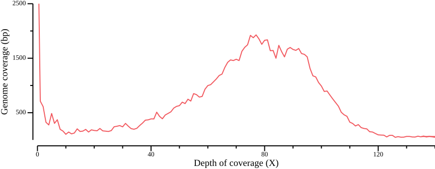

Figure 8: Zoomed in view of depth distribution for all sites.

Missingness

vcftools --gzvcf $VCF --missing-site --out $OUT 2>/dev/null
head -n 3 ${OUT}.lmiss
csvtk summary -t -f 6:min,6:q1,6:median,6:mean,6:q3,6:max ${OUT}.lmiss

CHR POS N_DATA  N_GENOTYPE_FILTERED N_MISS  F_MISS
LG4 1   20  0   6   0.3
LG4 2   20  0   4   0.2
F_MISS:min  F_MISS:q1   F_MISS:median   F_MISS:mean F_MISS:q3   F_MISS:max
0.00    0.00    0.10    0.16    0.20    1.00

csvtk plot hist --bins 20 -t -f F_MISS ${OUT}.lmiss > ${OUT}.lmiss.png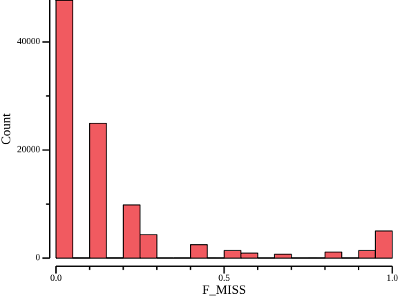

Figure 9: Distribution of missingness among all sites.

Filter input

Unless there is any strange bias that leads to a difference in coverage between variant and invariant sites, the final values should be similar to those before. We set filters and generate the output:

MISS=0.75
MIN_DEPTH=5
MAX_DEPTH=15

OUTVCF=${VCF%.subset.vcf.gz}.filtered.vcf.gz
vcftools --gzvcf $VCF \
   --remove-indels --max-missing $MISS \
   --min-meanDP $MIN_DEPTH --max-meanDP $MAX_DEPTH \
   --minDP $MIN_DEPTH --maxDP $MAX_DEPTH --recode \
   --stdout 2>/dev/null |
 gzip -c > $OUTVCF

Compare the results with the original input:

bcftools stats $OUTVCF | grep "^SN"

SN  0   number of samples:  10
SN  0   number of records:  46691
SN  0   number of no-ALTs:  43386
SN  0   number of SNPs: 2244
SN  0   number of MNPs: 0
SN  0   number of indels:   0
SN  0   number of others:   0
SN  0   number of multiallelic sites:   129
SN  0   number of multiallelic SNP sites:   43

Genotype depth data and BED output

Instead of calculating missing genotypes per site, we can retrieve the individual depth for each genotype with --geno-depth. Since we know cutoffs for mean depth (5-15), we can run this command on the main input file (allsites.vcf.gz). For reasons that soon will become clear, we also rerun --site-depth-mean.

VCF=allsites.vcf.gz
OUT=vcftools/allsites
vcftools --gzvcf  ${VCF} --geno-depth --out $OUT 2>/dev/null
vcftools --gzvcf  ${VCF} --site-mean-depth --out $OUT 2>/dev/null
head -n 3 ${OUT}.gdepth

CHROM   POS PUN-R-ELF   PUN-R-JMC   PUN-R-LH    PUN-R-MT    PUN-R-UCSD  PUN-Y-BCRD  PUN-Y-INJ   PUN-Y-LO    PUN-Y-PCT   PUN-Y-POTR
LG4 1   1   0   3   1   3   0   3   0   2   2
LG4 2   1   1   3   1   3   0   3   0   2   2

We could then combine these two files and perform filtering as follows: for each site check that

the mean depth is within the filter range
there is a minimimum number of genotypes with sufficient depth
individual genotype depth does not exceed a maximum depth threshold

If any of the points above fail, the site is discarded. We keep track of sites that pass the filters and output positions in BED format (a 0-based tab-separated format consisting of columns chrom, chromStart, and chromEnd).

Here is some code to achieve these goals. Unfortunately csvtk doesn’t seem to have support for calculating column margins out of the box, which is why we have to resort to this complicated construct using awk to count the number of individual genotypes that pass the coverage threshold 5.

BEDOUT=${VCF%.vcf.gz}.keep.bed
csvtk join -t ${OUT}.ldepth.mean ${OUT}.gdepth -f CHROM,POS |\
    csvtk filter -t -f "MEAN_DEPTH>=5" |\
    csvtk filter -t -f "MEAN_DEPTH<=15" |\
    awk -v FS="\t" -v OFS="\t" \
        'NR > 1 {count=0; for (i=4; i<=NF; i++)\
 {if ($i>4) count++ }; if (count>=5) print $1, $2 - 1, $2}'|\
    bedtools merge > ${BEDOUT}
head -n 3 $BEDOUT

LG4 76  99
LG4 278 336
LG4 346 409

The BED file contains a list of regions that are accessible to analysis.

Sequence masks

In addition to the BED output files, we can generate sequence masks. First, we set a variable to point to the reference sequence and index it.

export REF=M_aurantiacus_v1.fasta
samtools faidx ${REF}

Now, we use the command bedtools makefasta to make a sequence mask file in FASTA format consisting solely of 1’s:⁹

awk 'BEGIN {OFS="\t"} {print $1, 0, $2}' ${REF}.fai > ${REF}.bed
bedtools maskfasta -fi ${REF} -mc 1 -fo ${REF}.mask.fa -bed ${REF}.bed

We generate a file where all positions are masked because the BED files contain regions that we want to keep. Therefore, we want to convert corresponding positions to zeros. This file will be used as a template for all mask files.

We then apply bedtools maskfasta again to unmask (set to 0) the positions that overlap with the BED coordinates:

bedtools maskfasta -fi ${REF}.mask.fa -mc 0 -fo ${REF}.unmask.fa \
   -bed allsites.keep.bed
head -n 3 ${REF}.unmask.fa

>LG4
111111111111111111111111111111111111111111111111111111111111
111111111111111100000000000000000000000111111111111111111111

We can convince ourselves that this has worked by counting the number of unmasked positions in both the BED file (with bedtools genomecov) and sequence mask:

bedtools genomecov -i allsites.keep.bed -g ${REF}.fai | grep genome
# tr: -d deletes all characters not (-c, complement) in the character
# set '0'. wc: -m option counts characters
cat ${REF}.unmask.fa | tr -d -c '0' | wc -m

genome  0   20935   100000  0.20935
genome  1   79065   100000  0.79065
79065

Note that 0 and 1 in the bedtools genomecov output refers to coverage (i.e., absence/presence) and not unmask/mask as in the mask FASTA file.

Example: Using a sequence mask with `vcftools`

The sequence mask file can be used with vcftools with the option --mask. Before we use, however, we need to convert the mask file to one sequence per line¹⁰. seqkit is a neat tool that allows us to do this without hassle. As an example, we then perform a genetic diversity calculation with and without mask file to highlight the difference:

WIDEMASK=${REF}.unmask.wide.fa
seqkit seq -w 0 ${REF}.unmask.fa > ${WIDEMASK}
vcftools --gzvcf allsites.vcf.gz --mask $WIDEMASK \
         --site-pi --stdout 2>/dev/null |\
    csvtk summary -t --ignore-non-numbers --decimal-width 4 \
    --fields PI:count,PI:mean
vcftools --gzvcf allsites.vcf.gz --site-pi --stdout 2>/dev/null |\
    csvtk summary -t --ignore-non-numbers --decimal-width 4 \
    --fields PI:count,PI:mean

PI:count    PI:mean
79065   0.0183
PI:count    PI:mean
100000  0.0208

Clearly, filtering may have significant impact on the final outcome. You must choose your filters wisely!

Advanced depth filtering on BAM files

Important

This exercise is optional. It was created prior to the previous filtering exercises and may contain overlapping explanations and information. The procedure closely resembles that from the section on genotype depth data above, but depth profiles are now calculated from BAM files, which requires different tools.

In this section, we will restrict our attention to coverage-based filters, with the aim of generating sequence masks to denote regions of a reference sequence that contain sufficient information across individuals and populations. Furthermore, the masks will be applied in the context of genetic diversity calculations, in which case specific filters on polymorphic sites (e.g., p-value or minimum minor allele frequency (MAF)) should not be applied (all sites contain information).

Mapped reads provide information about how well a given genomic region has been represented during sequencing, and this information is usually summarized as the sequencing coverage. For any locus, this is equivalent to the number of reads mapping to that locus.

Sequencing coverage is typically not uniformly distributed over the reference. Reasons may vary but include uneven mapping coverage due to repeat regions, low coverage due to mis-assemblies, or coverage biases generated in the sequencing process. Importantly, both variable and monomorphic sites must be treated identically in the filtering process to eliminate biases between the two kinds of sites.

In this part, we will use mosdepth and bedtools to quickly generate depth of coverage profiles of mapped data. mosdepth is an ultra-fast command line tool for calculating coverage from a BAM file. By default, it generates a summary of the global distribution, and per-base coverage in bed.gz format. We will be using the per-base coverage for filtering.

Alternatively, mosdepth can also output results in a highly compressed format d4, which has been developed to handle the ever increasing size of resequencing projects. Files in d4 format can be processed with the d4-tools tool (Hou et al., 2021). For instance, d4tools view will display the coverage in bed format. We mention this in passing as it may be relevant when working with large genomes or sample sizes, but given the size of our sample data, we will be using bedtools from now on.

Per sample coverage

We start by calculating per-sample coverages with mosdepth. For downstream purposes, we need to save the size of the chromosomes we’re looking at, and for many applications, a fasta index file is sufficient.

export REF=M_aurantiacus_v1.fasta
samtools faidx ${REF}

The syntax to generate coverage information for a BAM file is mosdepth <prefix> <input file>. Here, we add the -Q option to exclude reads with a mapping quality less than 20:

mosdepth -Q 20 PUN-Y-INJ PUN-Y-INJ.sort.dup.recal.bam

The per-base coverage output file will be named PUN-Y-INJ.per-base.bed.gz and can be viewed with bgzip:

bgzip -c -d PUN-Y-INJ.per-base.bed.gz | head -n 5

LG4 0   9   3
LG4 9   13  4
LG4 13  53  5
LG4 53  56  6
LG4 56  62  7

To get an idea of what the coverage looks like over the chromsome, we will make use of two versatile programs for dealing with genomic interval data and delimited text files. Both programs operate on streams, enabling the construction of powerful piped commands at the command line (see below).

The first is bedtools, which consists of a set of tools to perform genome arithmetic on bed-like file formats. The bed format is a tab-delimited format that at its simplest consists of the three columns chrom (the chromosome name), chromStart, and chromEnd, the start and end coordinates of a region.

The second is csvtk, a program that provides tools for dealing with tab- or comma-separated text files. Avid R users will see that many of the subcommands are similar to those in the tidyverse dplyr package.

We can use these programs in a one-liner to generate a simple coverage plot (Figure 10)¹¹

bedtools intersect -a <(bedtools makewindows -g ${REF}.fai -w 1000) \
      -b PUN-Y-INJ.per-base.bed.gz -wa -wb | \
  bedtools groupby -i - -g 1,2,3 -c 7 -o mean | \
  csvtk plot -t line -x 2 -y 4 --point-size 0.01 --xlab Position \
      --ylab Coverage --width 9.0 --height 3.5 > fig-plot-coverage.png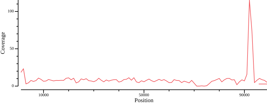

Figure 10: Coverage for sample PUN-Y-INJ in 1kb windows. Experiment changing the window size (`-w`) parameter to change smoothing.

Apparently there are some high-coverage regions that could be associated with, e.g., collapsed repeat regions in the assembly. Let’s compile coverage results for all samples, using bash string manipulation to generate file prefix¹²

# [A-Z] matches characters A-Z, * is a wildcard character that matches
# anything
for f in [A-Z]*.sort.dup.recal.bam; do
 # Extract the prefix by removing .sort.dup.recal.bam
 prefix=${f%.sort.dup.recal.bam}
 mosdepth -Q 20 $prefix $f
 # Print sample name
 echo -e -n "$prefix\t"
 # Get the summary line containing the total coverage
 cat $prefix.mosdepth.summary.txt | grep total
done > ALL.mosdepth.summary.txt
# View the file
cat ALL.mosdepth.summary.txt

PUN-R-ELF   total   100000  845166  8.45    0   187
PUN-R-JMC   total   100000  934032  9.34    0   244
PUN-R-LH    total   100000  940246  9.40    0   225
PUN-R-MT    total   100000  956272  9.56    0   233
PUN-R-UCSD  total   100000  812507  8.13    0   293
PUN-Y-BCRD  total   100000  882549  8.83    0   320
PUN-Y-INJ   total   100000  818921  8.19    0   229
PUN-Y-LO    total   100000  656112  6.56    0   151
PUN-Y-PCT   total   100000  836694  8.37    0   179
PUN-Y-POTR  total   100000  795201  7.95    0   205

We can calculate the total coverage by summing the values of the fifth column with csvtk as follows:

csvtk summary -H -t ALL.mosdepth.summary.txt -f 5:sum

to get the total coverage 84.78, which gives a hint at where the diploid coverage peak should be.

Sample set coverages

In this section, we will summarize coverage information for different sample sets, the motivation being that different filters may be warranted depending on what samples are being analysed. For instance, the coverage cutoffs for all samples will most likely be different from those applied to the subpopulations. In practice this means summing coverage tracks like those in Figure 10 for all samples.

We can combine the coverage output from different samples with bedtools unionbedg. We begin by generating a coverage file for all samples, where the output columns will correspond to individual samples. To save typing, we collect the sample names and generate matching BED file names to pass as arguments to options -names and -i, respectively. Also, we include positions with no coverage (-empty) which requires the use of a genome file (option -g). The BED output is piped to bgzip which compresses the output, before finally indexing with tabix¹³.

SAMPLES=$(csvtk grep -f Taxon -r -p "yellow" -r -p "red" sampleinfo.csv | csvtk cut -f SampleAlias | grep -v SampleAlias | tr "\n" " ")
BEDGZ=$(for sm in $SAMPLES; do echo -e -n "${sm}.per-base.bed.gz "; done)
bedtools unionbedg -header -names $SAMPLES -g ${REF}.fai -empty -i $BEDGZ | bgzip > ALL.bg.gz
tabix -f -p bed -S 1 ALL.bg.gz

Command line magic

The code above works as follows. We first use csvtk to grep (search) for the population names red and yellow in the Taxon column in sampleinfo.csv, thereby filtering the output to lines where Taxon matches the population names. Then, we cut out the interesting column SampleAlias and remove the header (grep -v SampleAlias matches anything but SampleAlias). Finally, tr translates newline character \n to space. The output is stored in the SAMPLES variable through the command substitution ($()) syntax.

We then iterate through the $SAMPLES to generate the input file names with the echo command, storing the output in $BEDGZ. These variables are passed on to bedtools unionbedg to generate a bedgraph file combining all samples.

As mentioned previously, we also need to combine coverages per populations yellow and red.

Exercise

Using the previous command as a template, try to generate per population coverage files.

Hint

You only need to modify the code that generates SAMPLES by grepping for each population separately (csvtk grep -f Taxon -r -p red and so on), or setting them manually. Remember also to modify the output file name (e.g., red.bg.gz).

Answer

An example using a for loop is shown here. You could copy-paste the code above and explicitly write out the population labels.

for pop in red yellow; do
 SAMPLES=$(csvtk grep -f Taxon -r -p $pop sampleinfo.csv | csvtk cut -f SampleAlias | grep -v SampleAlias | tr "\n" " ")
 BEDGZ=$(for sm in $SAMPLES; do echo -e -n "${sm}.per-base.bed.gz "; done)
 bedtools unionbedg -header -names $SAMPLES -g ${REF}.fai -empty -i $BEDGZ | bgzip > $pop.bg.gz
 tabix -f -p bed -S 1 $pop.bg.gz
done

Total coverage

Since we eventually want to filter on total coverage, we sum per sample coverages for each sample set with awk:

bgzip -c -d ALL.bg.gz | \
 awk -v FS="\t" -v OFS="\t" 'NR > 1 {sum=0; for (i=4; i<=NF; i++) sum+=$i; print $1, $2, $3, sum}' | \
 bgzip > ALL.sum.bed.gz
tabix -f -p bed ALL.sum.bed.gz

Here we use awk to sum from columns 4 and up (NF is the number of the last column).

For illustration, we plot the total coverage:

bedtools intersect -a <(bedtools makewindows -g ${REF}.fai -w 1000) \
    -b ALL.sum.bed.gz -wa -wb | \
  bedtools groupby -i - -g 1,2,3 -c 7 -o mean | \
  csvtk plot -t line -x 2 -y 4 --point-size 0.01 --xlab Position \
    --ylab Coverage --width 9.0 --height 3.5 > fig-plot-total-coverage.png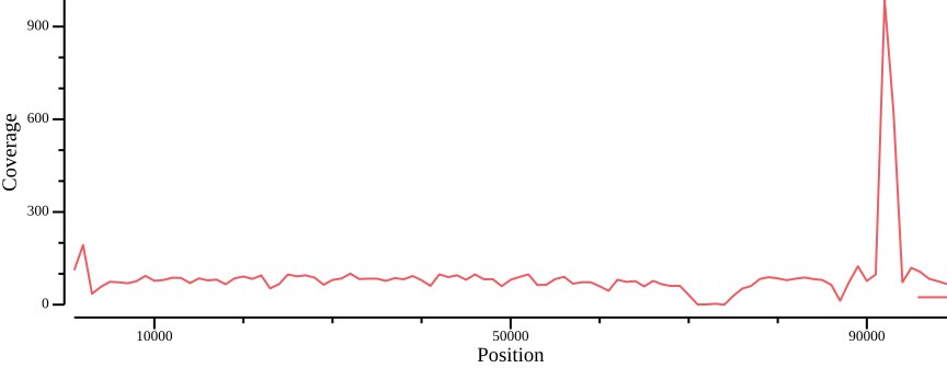

Figure 11: Total coverage in 1kb windows.

In order to define thresholds for subsequent filtering, we need to know the total coverage distribution. Therefore, we plot the proportion of the genome coverage versus depth of coverage (similar to k-mer plots in sequence assembly projects). To do so we must summarize our coverage file such that we count how many bases have a given coverage. This can be achieved by noting that each row in the BED file consists of the columns CHROM, START, END, and COVERAGE. We can generate a histogram table by, for each value of COVERAGE, summing the length of the regions (END - START).

# Add column containing length of region (end - start)
csvtk mutate2 -t -H -w 0 -e '$3-$2' ALL.sum.bed.gz | \
 # Sum the regions and *group* by the coverage (fourth column);
 # this gives the total number of bases with a given coverage
 csvtk summary -t -H -g 4 -f 5:sum -w 0 | \
 csvtk sort -t -k 1:n | \
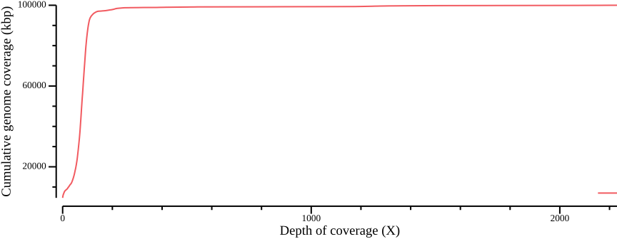
 awk -v cumsum=0 'BEGIN {OFS=","; cumsum=0} {cumsum += $2; print $1,$2,cumsum}' > ALL.sum.bed.csv

We plot the coverage distribution below, along with a plot of the cumulative coverage.

csvtk plot line -H ALL.sum.bed.csv -x 1 -y 2 --point-size 0.01 \
   --xlab "Depth of coverage (X)" --ylab "Genome coverage (bp)" \
   --width 9.0 --height 3.5 > fig-plot-total-coverage-distribution.png
csvtk plot line -H ALL.sum.bed.csv -x 1 -y 3 --point-size 0.01 \
   --xlab "Depth of coverage (X)" --ylab "Cumulative genome coverage (kbp)" \
   --width 9.0 --height 3.5 > fig-plot-total-coverage-distribution-cumulative.png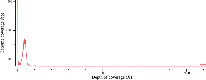

In Figure 12 a, a diploid peak is evident at around coverage X=100; we zoom in on that region to get a better view:

csvtk plot line -H ALL.sum.bed.csv -x 1 -y 2 --point-size 0.01 \
    --xlab "Depth of coverage (X)" --ylab "Genome coverage (bp)" \
    --width 9.0 --height 3.5 --x-min 40 --x-max 140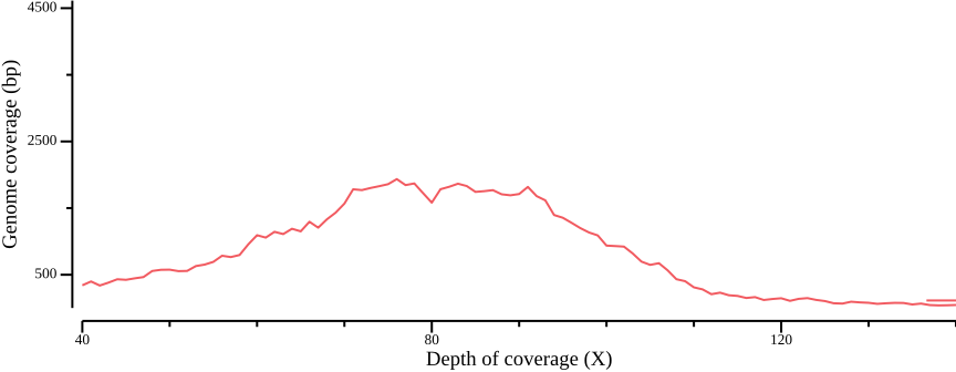

(Lou et al., 2021) point out that appropriate thresholds depend on the data set, but as a general rule recommend a minimum depth threshold at <0.8X average coverage, and a maximum depth threshold at mean coverage plus one or two standard deviations. For the sake of simplicity, you could here infer a cutoff simply by manually inspecting Figure 13; here, we will use the range 50-110.

We then use these thresholds to generate a BED file containing regions that are accessible, i.e., have sufficient coverage for downstream analyses. We also calculate the number of bases that pass the filtering criteria.

csvtk filter -t -H ALL.sum.bed.gz -f '4>50' | \
 csvtk filter -t -H -f '4<110' | \
 bgzip -c > ALL.sum.depth.bed.gz
bedtools genomecov -i ALL.sum.depth.bed.gz -g ${REF}.fai  | grep genome

Consequently, 75.2% of the genome is accessible by depth.

Exercise

Generate coverage sums for the red and yellow sample sets, and from these determine coverage thresholds and apply the thresholds to generate BED files with accessible regions.

Answer

We base the answer on the previous code.

for pop in red yellow; do
 bgzip -c -d $pop.bg.gz | \
  awk -v FS="\t" -v OFS="\t" 'NR > 1 {sum=0; for (i=4; i<=NF; i++) sum+=$i; print $1, $2, $3, sum}' | \
  bgzip > $pop.sum.bed.gz
 tabix -f -p bed $pop.sum.bed.gz
 csvtk mutate2 -t -H -w 0 -e '$3-$2' $pop.sum.bed.gz | \
 csvtk summary -t -H -g 4 -f 5:sum -w 0 | \
 csvtk sort -t -k 1:n | \
 awk -v cumsum=0 'BEGIN {OFS=","; cumsum=0} {cumsum += $2; print $1,$2,cumsum}' > $pop.sum.bed.csv
done

for pop in red yellow; do
cat ${pop}.sum.bed.csv | \
  csvtk plot line -x 1 -y 2 --point-size 0.01 \
    --xlab "Depth of coverage (X)" --ylab "Genome coverage (bp)" \
    --width 9.0 --height 3.5 --x-min 0 --x-max 100 > \
    fig-plot-total-coverage-distribution-hist-zoom-in-$pop.png
done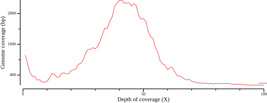

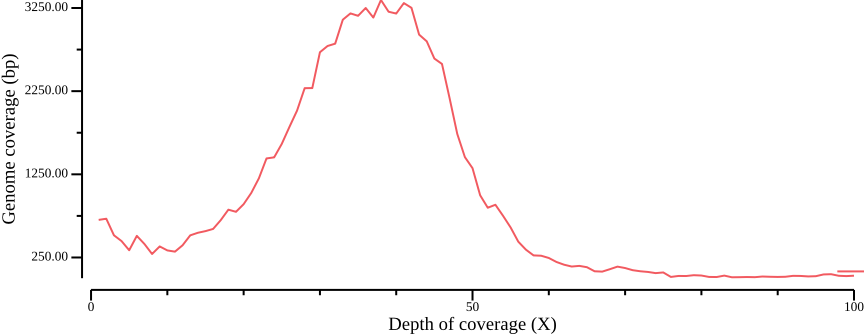
Based on Figure 14, we generate bed files with depths passing cutoffs:

# red filter: 20-60
csvtk filter -t -H red.sum.bed.gz -f '4>20' | \
 csvtk filter -t -H -f '4<60' | \
 bgzip -c > red.sum.depth.bed.gz
bedtools genomecov -i red.sum.depth.bed.gz -g ${REF}.fai  | grep genome

# yellow filter: 20-55
csvtk filter -t -H yellow.sum.bed.gz -f '4>20' | \
 csvtk filter -t -H -f '4<55' | \
 bgzip -c > yellow.sum.depth.bed.gz
bedtools genomecov -i yellow.sum.depth.bed.gz -g ${REF}.fai  | grep genome

genome  0   20853   100000  0.20853
genome  1   79147   100000  0.79147
genome  0   23231   100000  0.23231
genome  1   76769   100000  0.76769

Now we have combined total per sample coverage for ALL samples, and for sample sets red and yellow. The upcoming task will be to generate sequence masks from the total coverage and minimum number of individuals with coverage greater than zero.

Filter on minimum number of individuals

In addition to filtering on total coverage, we will also filter on the minimum number of individuals with a minimum depth. This is to account for cases where regions that pass the minimum coverage filter originate from just a few samples with unusually high coverage. Here, we will remove sites where more than 50% of individuals have zero coverage.

bgzip -c -d ALL.bg.gz | \
  awk -v FS="\t" 'BEGIN {OFS="\t"} NR > 1 {count=0; for (i=4; i<=NF; i++) {if ($i>0) count+=1}; if (count>=((NF-3)*0.5)) {print $1, $2, $3}}' | \
  bgzip > ALL.ind.bed.gz
tabix -f -p bed ALL.ind.bed.gz

Exercise

Use bedtools genomecov to determine the proportion of bases that are filtered out. Use ${REF}.fai as the argument to the required option -g.

Answer

bedtools genomecov -i ALL.ind.bed.gz -g ${REF}.fai

LG4 0   7694    100000  0.07694
LG4 1   92306   100000  0.92306
genome  0   7694    100000  0.07694
genome  1   92306   100000  0.92306

Exercise

Generate coverage sums for red and yellow sample sets.

Answer

for pop in red yellow; do
  bgzip -c -d $pop.bed.gz | awk -v FS="\t" 'BEGIN {OFS="\t"} NR > 1 {count=0; for (i=4; i<=NF; i++) {if ($i>0) count+=1}; if (count>=((NF-3)*0.5)) {print $1, $2, $3}}' | bgzip > $pop.ind.bed.gz
  tabix -f -p bed $pop.ind.bed.gz
done

[bgzip] Could not open red.bed.gz: No such file or directory
[bgzip] Could not open yellow.bed.gz: No such file or directory

Sequence masks

Finally, as before, we can convert the BED output to sequence mask files in FASTA format. Recall that we first have to make a template genome mask file where all positions are masked:

awk 'BEGIN {OFS="\t"} {print $1, 0, $2}' ${REF}.fai > ${REF}.bed
bedtools maskfasta -fi ${REF} -mc 1 -fo ${REF}.mask.fa -bed ${REF}.bed

Then, for each sample set, we will use bedtools intersect to intersect the BED files corresponding to the total sum coverage and the filter on number of individuals. bedtools intersect makes it easy to combine multiple BED files, so any other filters, or genomic features such as exons, could be added to make a compound mask file. The resulting BED files is used as input to bedtools maskfasta.

bedtools intersect -a ALL.sum.depth.bed.gz -b ALL.ind.bed.gz \
   -g ${REF}.fai | bgzip > ALL.unmask.bed.gz
tabix -f -p bed ALL.unmask.bed.gz
bedtools maskfasta -fi ${REF}.mask.fa -mc 0 -fo ${REF}.unmask.fa \
   -bed ALL.unmask.bed.gz
head -n 3 ${REF}.unmask.fa

>LG4
111111111111111111111111111111111111111111111111111111111111
111111111111111111100000000000000000000000000000000111111111

We can once again convince ourselves that this has worked by counting the number of unmasked positions:

# tr: -d deletes all characters not (-c, complement) in the character
# set '0'. wc: -m option counts characters
cat ${REF}.unmask.fa | tr -d -c '0' | wc -m
bedtools genomecov -i ALL.unmask.bed.gz -g ${REF}.fai | grep genome

75236
genome  0   24764   100000  0.24764
genome  1   75236   100000  0.75236

Note that 0 and 1 in the bedtools genomecov output refers to coverage (i.e., absence/presence) and not unmask/mask as in the mask FASTA file.

Exercise

Create unmask files for red and yellow populations.

Answer

for pop in red yellow; do
 bedtools intersect -a $pop.sum.depth.bed.gz -b $pop.ind.bed.gz \
    -g ${REF}.fai | bgzip > $pop.unmask.bed.gz
 tabix -f -p bed $pop.unmask.bed.gz
 bedtools maskfasta -fi ${REF}.mask.fa -mc 0 -fo ${REF}.$pop.unmask.fa \
    -bed $pop.unmask.bed.gz
done

Conclusion

Congratulations! You have now gone through a set of tedious and complex steps to generate output files that determine what regions in a reference DNA sequence are amenable to analysis. In the next exercise we will use these files as inputs to different programs that calculate diversity statistics from population genomic data.

References

Danecek, P., Auton, A., Abecasis, G., Albers, C. A., Banks, E., DePristo, M. A., Handsaker, R. E., Lunter, G., Marth, G. T., Sherry, S. T., McVean, G., & Durbin, R. (2011). The variant call format and VCFtools. Bioinformatics (Oxford, England), 27(15), 2156–2158. https://doi.org/10.1093/bioinformatics/btr330

Danecek, P., Bonfield, J. K., Liddle, J., Marshall, J., Ohan, V., Pollard, M. O., Whitwham, A., Keane, T., McCarthy, S. A., Davies, R. M., & Li, H. (2021). Twelve years of SAMtools and BCFtools. GigaScience, 10(2), giab008. https://doi.org/10.1093/gigascience/giab008

Garrison, E., Kronenberg, Z. N., Dawson, E. T., Pedersen, B. S., & Prins, P. (2022). A spectrum of free software tools for processing the VCF variant call format: Vcflib, bio-vcf, Cyvcf2, hts-nim and slivar. PLOS Computational Biology, 18(5), e1009123. https://doi.org/10.1371/journal.pcbi.1009123

Hou, H., Pedersen, B., & Quinlan, A. (2021). Balancing efficient analysis and storage of quantitative genomics data with the D4 format and D4tools. Nature Computational Science, 1(6), 441–447. https://doi.org/10.1038/s43588-021-00085-0

Li, H. (2014). Toward better understanding of artifacts in variant calling from high-coverage samples. Bioinformatics, 30(20), 2843–2851. https://doi.org/10.1093/bioinformatics/btu356

Lou, R. N., Jacobs, A., Wilder, A. P., & Therkildsen, N. O. (2021). A beginner’s guide to low-coverage whole genome sequencing for population genomics. Molecular Ecology, 30(23), 5966–5993. https://doi.org/10.1111/mec.16077

Maruki, T., & Lynch, M. (2017). Genotype Calling from Population-Genomic Sequencing Data. G3 Genes|Genomes|Genetics, 7(5), 1393–1404. https://doi.org/10.1534/g3.117.039008

Nielsen, R., Paul, J. S., Albrechtsen, A., & Song, Y. S. (2011). Genotype and SNP calling from next-generation sequencing data. Nature Reviews Genetics, 12(6), 443–451. https://doi.org/10.1038/nrg2986

Pedersen, B. S., & Quinlan, A. R. (2018). Mosdepth: Quick coverage calculation for genomes and exomes. Bioinformatics, 34(5), 867–868. https://doi.org/10.1093/bioinformatics/btx699

Purcell, S., Neale, B., Todd-Brown, K., Thomas, L., Ferreira, M. A. R., Bender, D., Maller, J., Sklar, P., de Bakker, P. I. W., Daly, M. J., & Sham, P. C. (2007). PLINK: A Tool Set for Whole-Genome Association and Population-Based Linkage Analyses. The American Journal of Human Genetics, 81(3), 559–575. https://doi.org/10.1086/519795

Quinlan, A. R., & Hall, I. M. (2010). BEDTools: A flexible suite of utilities for comparing genomic features. Bioinformatics, 26(6), 841–842. https://doi.org/10.1093/bioinformatics/btq033

Shen, W., Le, S., Li, Y., & Hu, F. (2016). SeqKit: A Cross-Platform and Ultrafast Toolkit for FASTA/Q File Manipulation. PLOS ONE, 11(10), e0163962. https://doi.org/10.1371/journal.pone.0163962

Footnotes

The password is provided by the course instructor↩︎
This exercise is inspired by and based on https://speciationgenomics.github.io/filtering_vcfs/]↩︎
We select a fix number that should contain enough information to generate reliable statistics. This number should not change significantly even when files contain vastly different numbers of sites, which is why we need adjust the parameter r to the number of sites in the file.↩︎
vcftools does not have a -h or --help option.↩︎
The 2>/dev/null outputs messages from vcftools to a special file /dev/null which is a kind of electronic dustbin.↩︎
On viewing csvtk plots: either you can redirect (>) the results from csvtk to a png output file, or you can pipe (|) it to the command display (replace > $OUT.ldepth.png by | display, which should fire up a window with your plot.↩︎
You can try different values of the --bins option↩︎
Purcell et al. (2007), p. 565 gives a coherent derivation of this estimator↩︎
We need to generate a BED file representation of the FASTA index unfortuanely as bedtools makefasta doesn’t handle FASTA indices natively.↩︎
For vcftools; unfortunate, but that’s the way it is↩︎
The one-liner combines the results of several commands in a pipe stream. Also, Bash redirections are used to gather the results from the output of bedtools makewindows to bedtools intersect. The intersection commands collects coverage data in 1kb windows that are then summarized by bedtools groupby.↩︎
The % operator deletes the shortest match of $substring from back of $string: ${string%substring}. See Bash string manipulation for more information.↩︎
Instead of using the command substitution, you could look into the sample info file and set the sample names manually: SAMPLES="PUN-Y-BCRD PUN-R-ELF PUN-Y-INJ PUN-R-JMC PUN-R-LH PUN-Y-LO PUN-R-MT PUN-Y-PCT PUN-Y-POTR PUN-R-UCSD"↩︎

Background

Some recommended data filters

Basic filtering of a VCF file2

Generate random subset of variants

Generate statistics for filters

Total depth per site

Variant quality distribution

Minor allele frequency distribution

Missing data for individuals and sites

Heterozygosity

Filtering the VCF

Depth filtering of VCF with invariant sites

Data summary and subset

Data for depth filters

allsites subset

Depth per site

Missingness

Filter input

Genotype depth data and BED output

Sequence masks

Example: Using a sequence mask with vcftools

Advanced depth filtering on BAM files

Per sample coverage

Sample set coverages

Total coverage

Filter on minimum number of individuals

Sequence masks

Conclusion

References

Footnotes

Basic filtering of a VCF file²

Example: Using a sequence mask with `vcftools`