The range is the difference between the largest and the smallest observations in the data set. Similar to mean, it can be a misleading measure if there are outliers in the data.
If we arrange the data in order of magnitude, starting with the smallest and ending with the largest value we can define percentiles. The value of \(x\) that has 1% of the observations in the ordered set lying below it (and 99% of the observations lying above it) is called the 1st percentile. The value of \(x\) that has 2% of the observations in the ordered set lying below it (and 98% of the observations lying above it) is called the 2nd percentile, and so on. The values of \(x\) that divide the ordered set into 10 equally sized groups, that is the 10th, 20th, 30th, …, 90th percentiles, are called deciles.
Quartiles are the three values that divide the data values into four equally sized groups.
Q1. Lower quartile. 25% of values are below Q1. Divides the values below the median into equally sized groups.
Q2. Median. 50% of values are below Q2 and 50% are above Q2. Q2 is the median that we have seen before.
Q3. Upper quartile. 75% of values are below Q3. Divides the values above the median into equally sized groups.
Going back to the diabetes data set, what are the three quartiles of participants age?
The interquartile range, IQR, is the difference between the 1st (Q1) and the 3rd (Q3) quartiles, i.e. between the 25th and 75th percentiles. It contains the central 50% of the observations in the ordered set.
\[IQR = Q3 - Q1\]
For instance, the IQR range for age value for our study is:
iqr = Q3 - Q1print(iqr)
[1] 21.75
7.4 Variance and standard deviation
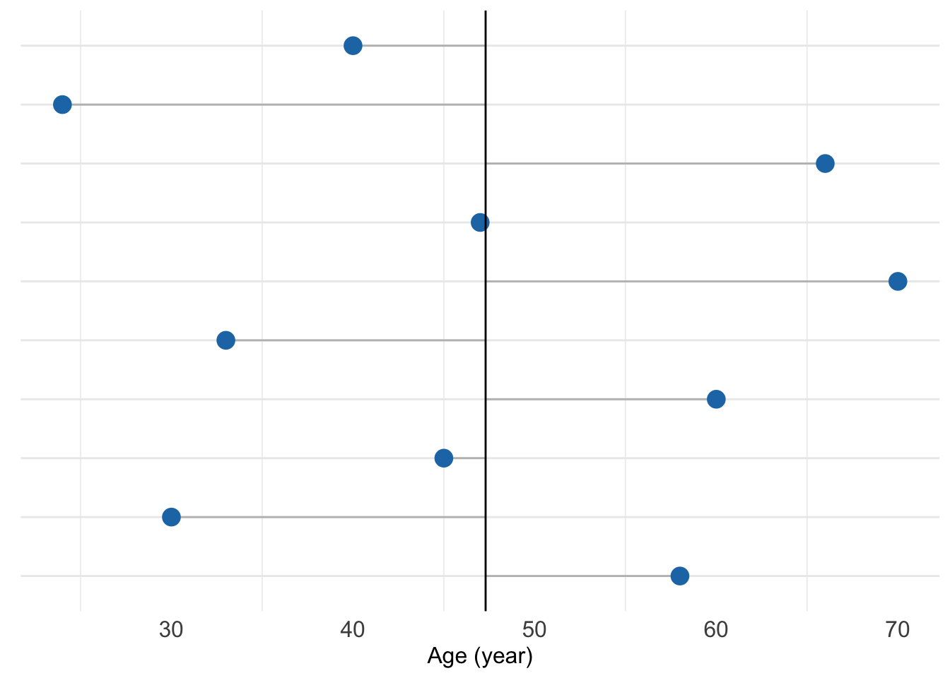
The variance of a set of observations is their mean squared distance from the mean value:
Figure 7.1: First ten age measurements for the study participants. Grey lines show the distance to the age mean value.
The variance is measured in the square of the unit in which \(x\) was measured. Another common measure using the same unit as \(x\) is standard deviation, defined as the square root of the variance:
Typically, we regard the collection of observations \(x_1, \dots, x_n\) as a sample drawn from a large population of possible observations. It has been shown theoretically that we obtain a better sample estimate of the population variance and standard deviation if we divide by \((n-1)\). So the denominator \(n\) is commonly replaced by \(n-1\) and the sample variance is calculated instead as
we calculate standard deviation, \(\sigma\), when we consider our observations to be entire population (Equation 7.2)
we calculate sample standard deviation, \(s\), when we consider our observations a random sample from a larger population, as a better estimate of the standard deviation of the larger population (Equation 7.4)
Let’s calculate variance, standard deviation and sample standard deviation for age.
# extract age valuesage <- data_diabetes %>%pull(age)# number of observationsn <-length(age)# calculate mean (arithmetic)age_mean <-mean(age)# calculate variance following variance equationsigma2 <- (sum((age - age_mean)^2))/(n)# calculate standard deviation following standard deviation equationsigma <-sqrt((sum((age - age_mean)^2))/(n))# calculate sample variance following sample variance equations2 <- (sum((age - age_mean)^2))/(n-1)# calculate sample standard deviation following sample standard deviation equations <-sqrt((sum((age - age_mean)^2))/(n-1))# collect resultsv.name <-c("sigma2", "sigma", "s2", "s")v.values <-c(sigma2, sigma, s2, s)results <-data.frame(stats = v.name, value = v.values)print(results)## stats value## 1 sigma2 224.80828## 2 sigma 14.99361## 3 s2 226.55098## 4 s 15.05161
We can check our calculations of sample variance and sample standard deviation using R functions var() and sd()
There are naturally additional measure of spread and to assess the shape of data distribution. Some examples include the Coefficient of Variation (CV), calculated as the ratio of the standard deviation to the mean. CV is commonly used to compare the variability of measurements across different groups or conditions in biological experiments, regardless of their units. The Mean Absolute Deviation (MAD) measures average deviation from the mean, offering a robust alternative to the standard deviation, particularly useful in studies with outliers, such as enzyme kinetics where reaction rates can vary widely. Skewness measures the asymmetry of a distribution around its mean, important in clinical data to determine if results are biased toward high or low values, which might indicate non-normal behavior like skewed immune response. Kurtosis evaluates the ‘tailedness’ of the distribution; in pharmacological data, high kurtosis might suggest a concentration of data around a mean with extreme outliers, indicative of varying drug responses among patients.
Coefficient of Variation (CV)\[\text{CV} = \frac{\sigma}{\mu} \times 100\%\] Here, \(\sigma\) is the standard deviation and \(\mu\) is the mean of the dataset. The CV is expressed as a percentage to indicate the ratio of the standard deviation to the mean.
Mean Absolute Deviation (MAD)\[\text{MAD} = \frac{1}{n} \sum_{i=1}^{n} |x_i - \mu|\] This represents the average of the absolute differences between each data point \(x_i\) and the mean \(\mu\) of the dataset, where \(n\) is the number of observations.
Skewness\[\text{Skewness} = \frac{n}{(n-1)(n-2)} \sum_{i=1}^{n} \left(\frac{x_i - \mu}{\sigma}\right)^3\] Skewness measures the asymmetry of the data around the mean. Positive skew indicates a tail on the right side of the distribution, and negative skew indicates a tail on the left.
Kurtosis\[\text{Kurtosis} = \frac{n(n+1)}{(n-1)(n-2)(n-3)} \sum_{i=1}^{n} \left(\frac{x_i - \mu}{\sigma}\right)^4 - \frac{3(n-1)^2}{(n-2)(n-3)}\] Kurtosis assesses the tailedness of the distribution. A higher kurtosis than the normal distribution (which has a kurtosis of 3) indicates a distribution with more pronounced tails.