5  Numerical data

Code

# load libraries
library(tidyverse)
library(kableExtra)
library(faraway)
library(scales)
library(ggbeeswarm)
library(gridExtra)

# define generic ggplot theme
font.size <- 12
col.blue.light <- "#a6cee3"
col.blue.dark <- "#1f78b4"
my.ggtheme <- theme(axis.title = element_text(size = font.size), 
        axis.text = element_text(size = font.size), 
        legend.text = element_text(size = font.size), 
        legend.title = element_blank(), 
        legend.position = "top", 
        axis.title.y = element_text(angle = 0)) 

# add obesity and diabetes status to diabetes faraway data
inch2m <- 2.54/100
pound2kg <- 0.45
data_diabetes <- diabetes %>%
  mutate(height  = height * inch2m, height = round(height, 2)) %>% 
  mutate(waist = waist * inch2m) %>%  
  mutate(weight = weight * pound2kg, weight = round(weight, 2)) %>%
  mutate(BMI = weight / height^2, BMI = round(BMI, 2)) %>% 
  mutate(obese= cut(BMI, breaks = c(0, 29.9, 100), labels = c("No", "Yes"))) %>% 
  mutate(diabetic = ifelse(glyhb > 7, "Yes", "No"), diabetic = factor(diabetic, levels = c("No", "Yes"))) %>%
  na.omit()

Numerical data, both discrete and continuous, can be visualized and summarized in many ways. Common plots include histograms, density plots and scatter plots. Summary statistics include measures of location such as mode and median and measures of spread such as variance or median absolute deviation. It is also common to visualize summary statistics, e.g. on box plot.

flowchart TD
  A(Numerical data) --> B(Numerical summary)
  A(Numerical data) --> C(Graphical summary)
  B(Numerical summary) --> D(Measures of location <br/> e.g. mode, average, median)
  B --> E(Measures of spread <br/> e.g. quartiles, variance, standard deviation)
  C(Graphical summary) --> F(Histogram <br/> Density plot <br/> Box plot <br/> ...)

Figure 5.1: Example of numerical summaries and graphical visualization applicable to numerical data

5.1 Strip plot, Jittered strip plot & Beeswarm plot

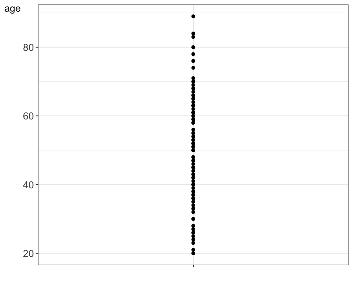
When the data set is not very big, i.e. does not contain millions of measurements for a given numerical variable of interest, it is recommended to visually assess all measurements on a plot. This can be done in a 1D scatter plot, called also a strip plot or a dot plot.

For instance the age values for the 130 participants in the diabetes study are:

Code

print(data_diabetes$age)

  [1] 58 30 45 60 33 70 47 66 24 40 42 61 61 70 36 55 65 20 74 51 71 76 40 40 76
 [26] 48 64 21 47 61 65 41 50 83 26 53 50 48 59 63 43 58 59 35 50 27 67 51 51 59
 [51] 58 66 43 65 34 37 61 45 68 63 55 66 63 78 68 61 63 54 50 51 45 38 63 50 44
 [76] 48 69 62 36 47 23 38 40 40 60 63 63 46 56 43 26 30 36 44 63 28 52 53 30 45
[101] 35 50 27 52 42 39 28 53 55 84 80 60 80 63 37 20 54 58 52 33 37 32 60 42 52
[126] 25 37 89 53 51

Let’s visualize these age values using a strip plot.

Code

# plot strip plot
data_diabetes %>%
  ggplot(aes(x = "", y = age)) + 
  geom_point() + 
  theme_bw() + 
  ylab("age") + 
  xlab("") + 
  my.ggtheme

Figure 5.2: A strip plot showing age values for the 130 study participants

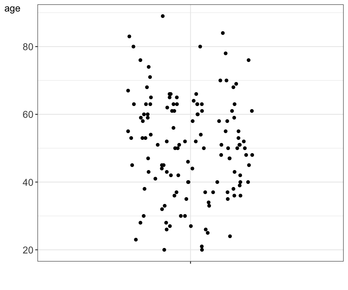
As year was recorded in years and we have over 100 participants, it happens that some age values are repeated, e.g. we have 2 participants who were 20 years old and 3 that were 30 years old at the time of study. These repeated measurements are shown on top of each other and we cannot see them all. A jittered strip plot attempts to reduce such overlays by randomly moving data points by small amounts to the left and right.

Code

# plot jittered strip plot
data_diabetes%>%
  ggplot(aes(x = "", y = age)) + 
  geom_jitter(height = 0, width = 0.25) + 
  theme_bw() + 
  ylab("age") + 
  xlab("") + 
  my.ggtheme

Figure 5.3: A jittered strip plot showing age values for the 130 study participants

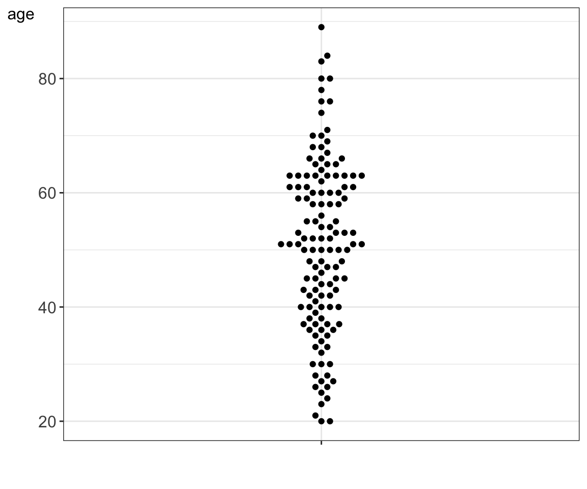
In a jittered strip plot some overlays may still occur, as the data points are moved at random. Further, many data points are moved unnecessarily. In a beeswarm plot data points are moved only when necessary, and even then the data point is only moved by the minimum distance required to avoid overlays.

Code

# plot beeswarm
data_diabetes %>%
  ggplot(aes(x = "", y = age)) + 
  geom_beeswarm(cex = 2) + 
  theme_bw() + 
  ylab("age") + 
  xlab("") + 
  my.ggtheme

Figure 5.4: A beeswarm showing age values for the 130 study participants

5.2 Histogram & density plot

A histogram bins the data and counts the number of observations that fall into each bin.

Code

# plot histogram
data_diabetes %>%
  ggplot(aes(x = age)) + 
  geom_histogram(binwidth = 5, center = 32.5, color = "white", fill = col.blue.dark) + 
  theme_bw() + 
  xlab("age") + 
  my.ggtheme

Figure 5.5: A histogram summarizing age values for the 130 study participants

A density plot is like a smoothed histogram where the total area under the curve is set to 1. A density plot is an approximation of a distribution.

Code

# plot density plot
data_diabetes %>% ggplot(aes(x = age)) + 
  geom_density() + 
  theme_bw() + 
  xlab("age") + 
  my.ggtheme

Figure 5.6: A density plot of age values for the 130 study participants

5.3 Histogram & density plot stratified by group

Code

# plot histogram
p.hist <- data_diabetes %>%
  ggplot(aes(x=age, fill=gender)) + 
  geom_histogram(bins=15, color="white", alpha = 0.6) + 
  xlab("age") + 
  theme_bw() + 
  scale_fill_brewer(palette = "Dark2") + 
  my.ggtheme

p.density <- data_diabetes %>%
  ggplot(aes(x=age, fill=gender)) + 
  geom_density(alpha = 0.6) + 
  xlab("age") + 
  theme_bw() + 
  scale_fill_brewer(palette = "Dark2") + 
  my.ggtheme

grid.arrange(arrangeGrob(p.hist, p.density, ncol=2))

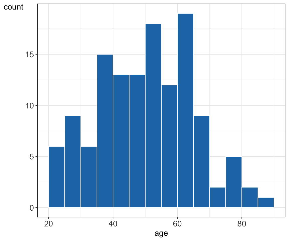
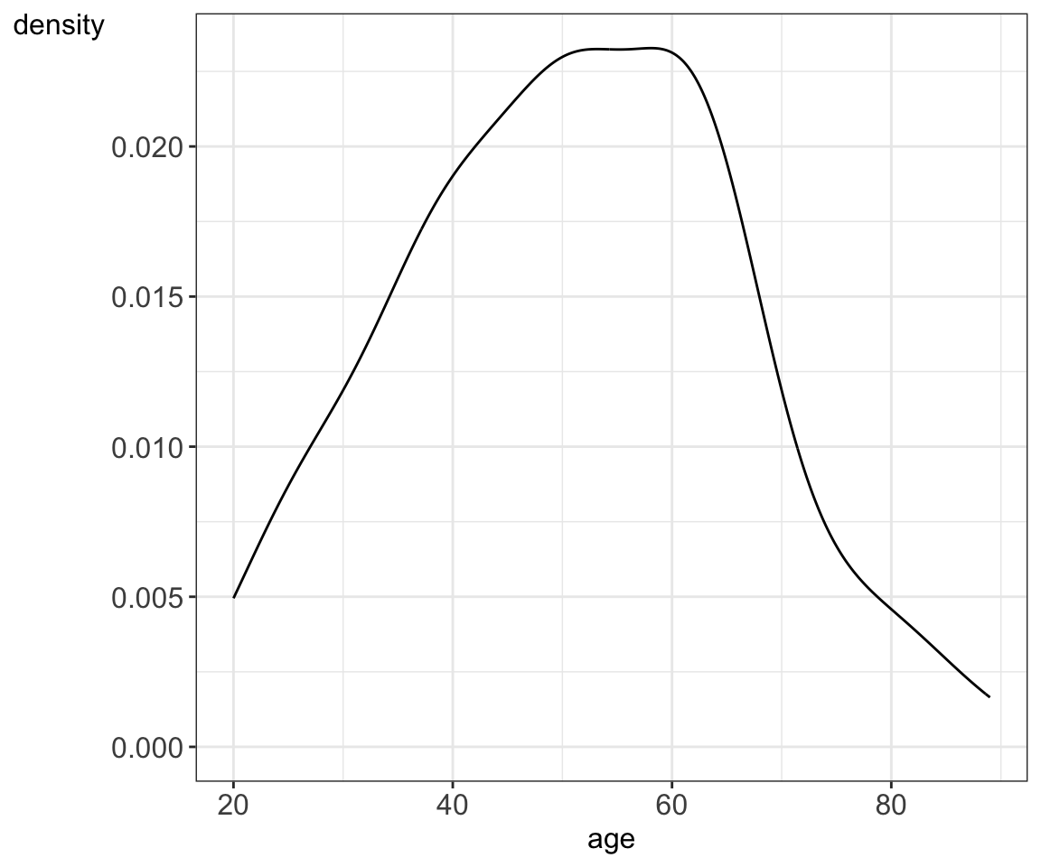
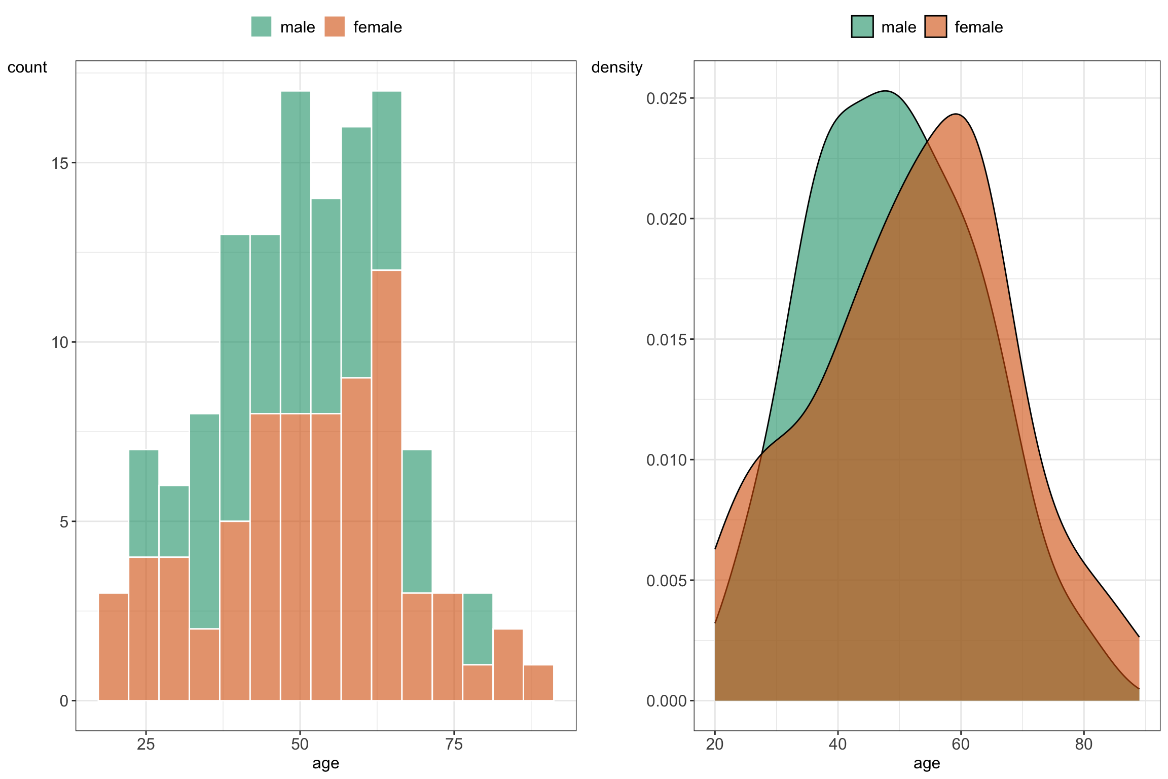
Figure 5.7: Histogram and density plots summarizing age values stratified by gender

5.4 Scatter plot: 2 numerical variables

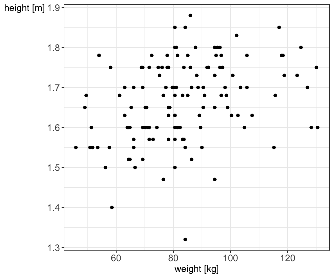
Scatter plots are useful when studying a relationship (association) between two numerical variables. Let’s look at the weight and height for our 130 study participants.

Code

# plot scatter plot
data_diabetes %>%
  ggplot(aes(x = weight, y = height)) + 
  geom_point() + 
  xlab("weight [kg]") + 
  ylab("height [m]") + 
  theme_bw() + 
  my.ggtheme

Figure 5.8: Scatter plot showing a relationship between weight and height

Code

# plot scatter plot
data_diabetes %>%
  ggplot(aes(x = weight, y = height, color = gender)) +
  geom_point() +
  xlab("weight [kg]") +
  ylab("height [m]") +
  theme_bw() +
  scale_color_brewer(palette = "Dark2") +
  my.ggtheme

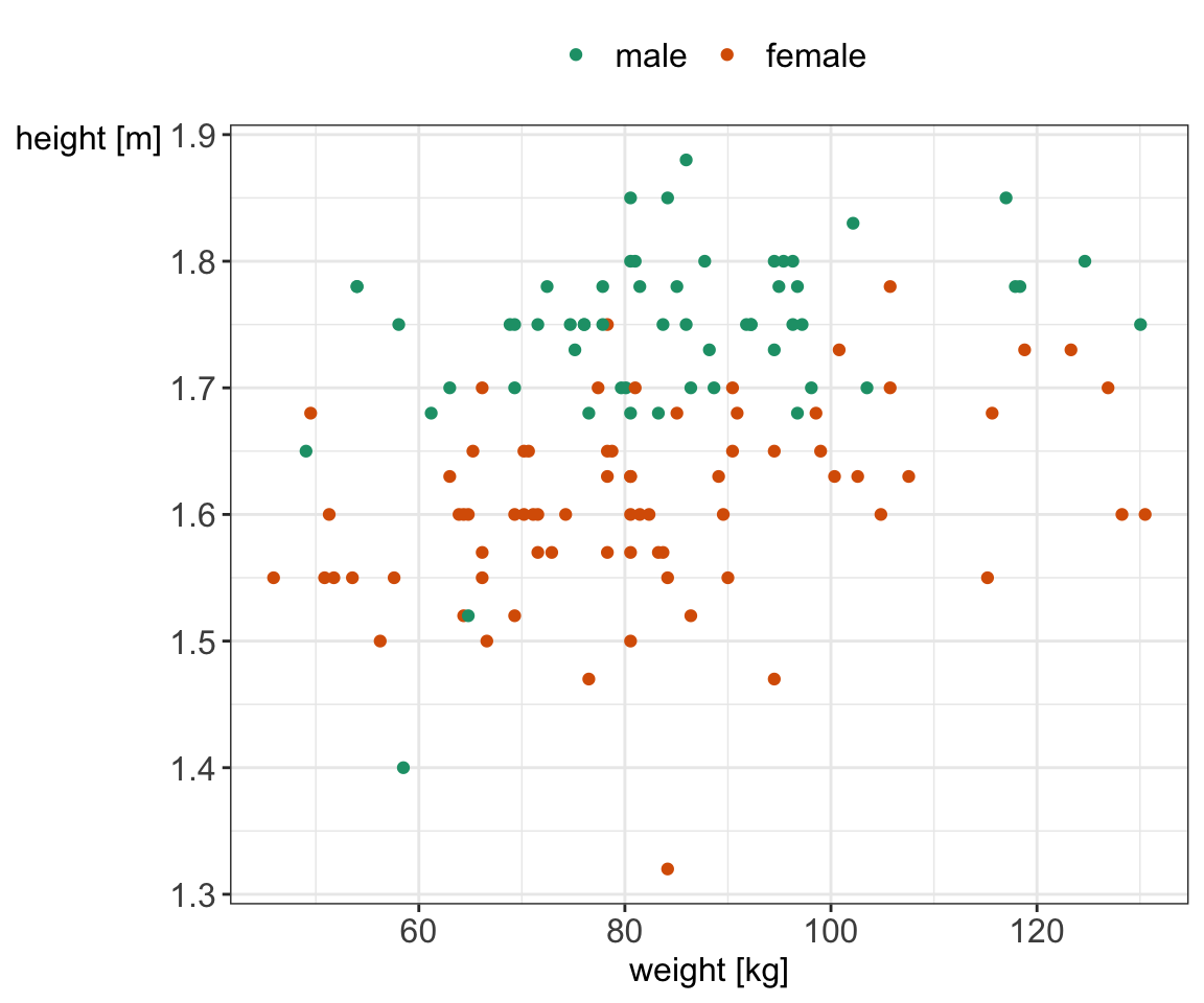
Figure 5.9: Scatter plot showing a relationship between weight and height stratified by gender

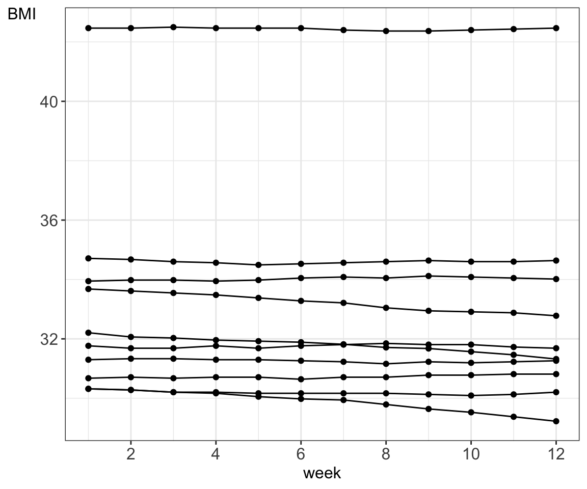
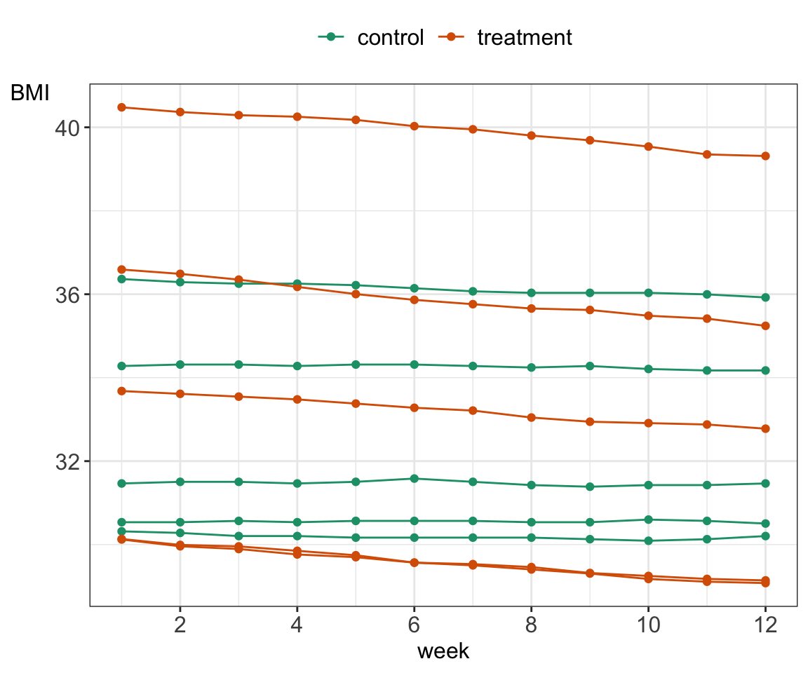
Sometimes, it is useful to connect the observations in the order in which they appear, e.g. when analyzing time series data. The diabetes data set does not contain any measurements over time but we can simulate some BMI values over time for demonstration purposes.

Code

# simulate BMI over time
# select participants with BMI >= 30
# assign half to control group and half to treatment to reduce weight 
# add simulated weight loss values to treatment group ca. 0.2 kg per week
# add simulated weight fluctuations, ca plus / minus 0.1 kg per week

data_diabetes_bmi30 <- data_diabetes %>% 
  filter(BMI >= 30) %>%
  select(id, weight, height, BMI) %>%
  mutate(group=sample(c("control", "treatment"), size=n(), replace=TRUE))

# add 52 weeks of simulated BMI values

no_weeks <- 12
weight_sim <- matrix(data = NA, 
                     nrow = nrow(data_diabetes_bmi30), 
                     ncol = no_weeks, 
                     dimnames = list(data_diabetes_bmi30$id, paste("week", 1: no_weeks, sep=""))) # initiate matrix to store simulated BMI values
weight_sim[, 1] <- data_diabetes_bmi30$weight # first column: baseline weight

for (n in 1:nrow(data_diabetes_bmi30)){
  
  for (p in 2:ncol(weight_sim)){
    
    # if control group: just fluctuate weight by random values between 0 and 0.2 kg
    # if treatment: decrease by random values between 0.1 and 0.5 kg from
    
    if (data_diabetes_bmi30$group[n] == "treatment"){
     
      loss <- runif(1, 0.1, 0.5) %>% round(1)
      weight_sim[n, p] <- weight_sim[n, p-1] - loss
      
    } else{
      
      fluctuation <- runif(1, -0.2, 0.2) %>% round(1)
      weight_sim[n, p] <- weight_sim[n, p-1] + fluctuation
      
    }
  
  }
}

# convert to tibble
weight_sim <- weight_sim %>%
  as_tibble(rownames = "id") %>%
  mutate(id = as.numeric(id))

# join data_diabetes_bmi30 with simulated
# keep 5 treatment and 5 control participants
data_diabets_sim <- data_diabetes_bmi30 %>%
  as_tibble() %>% 
  left_join(weight_sim, by = "id")

# plot BMI over time
data_plot <- data_diabets_sim %>%
  slice_sample(n = 10) %>%
  select(-weight, -BMI) %>% 
  pivot_longer(-c("id", "group", "height"), names_to = "week", values_to = "weight") %>% 
  mutate(BMI = weight / (height^2)) %>%
  mutate(week = gsub("week", "", week)) %>%
  mutate(week = as.numeric(week)) 

data_plot %>%
  ggplot(aes(x = week, y = BMI, group = id)) + 
  geom_point() +
  geom_line() + 
  xlab("week") +
  ylab("BMI") +
  theme_bw() +
  scale_color_brewer(palette = "Dark2") +
  scale_x_continuous(breaks= pretty_breaks()) + 
  my.ggtheme

Figure 5.10: A line plot for BMI simulated values over 12 weeks for 10 randomly selected study participants

Code

data_plot <- data_diabets_sim %>%
  group_by(group) %>%
  slice_sample(n = 5) %>%
  select(-weight, -BMI) %>% 
  pivot_longer(-c("id", "group", "height"), names_to = "week", values_to = "weight") %>% 
  mutate(BMI = weight / (height^2)) %>%
  mutate(week = gsub("week", "", week)) %>%
  mutate(week = as.numeric(week)) 

data_plot %>%
  ggplot(aes(x = week, y = BMI, group = id, colour = group)) + 
  geom_point() +
  geom_line() + 
  xlab("week") +
  ylab("BMI") +
  theme_bw() +
  scale_color_brewer(palette = "Dark2") +
  scale_x_continuous(breaks= pretty_breaks()) + 
  my.ggtheme

Figure 5.11: A line plot for BMI simulated values over 12 weeks for 5 randomly selected study participants from control and treatment group