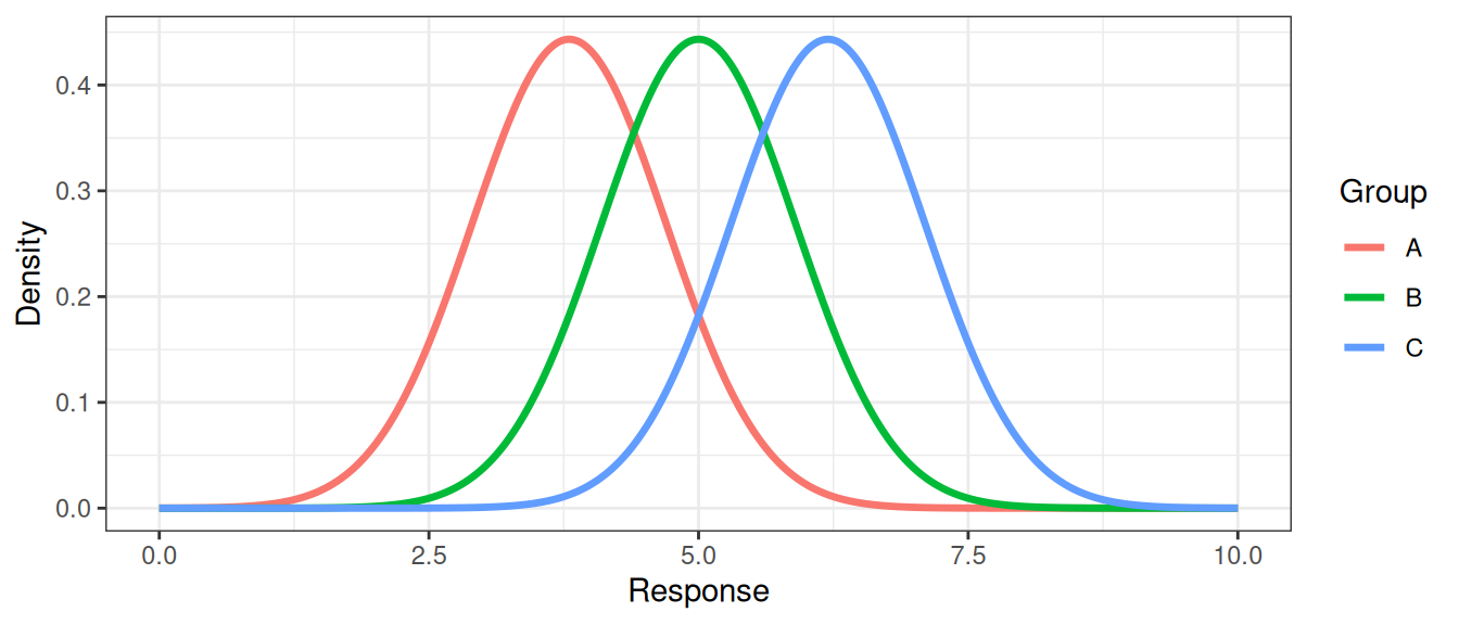
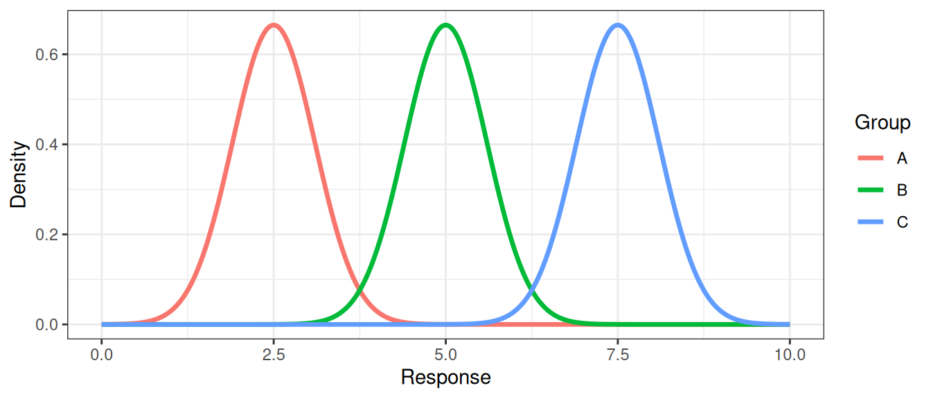
In previous sections, we have seen how to compare two groups using t-tests. However, sometimes we want to compare more than two groups. One way to do this is to perform multiple pairwise t-tests, but this approach has some limitations, such as inflating the Type I error rate. An omnibus test, such as analysis of variance (ANOVA), can be used to test for differences among multiple groups in a single test.
With one numeric response variable of interest, such as blood pressure or biomarker concentration, and one categorical variable with \(k\) groups, such as treatment group, we can use one-way ANOVA to test if the group means are equal.
Hypotheses: \[H_0: \mu_1=\mu_2=\cdots=\mu_k\] \[H_1: \text{not all group means are equal}\]
The ANOVA test statistic is based on the ratio of the variation between groups to the variation within groups. If the between-group variation is large relative to the within-group variation, we have evidence against the null hypothesis.
\[F = \frac{\text{variation between groups}}{\text{variation within groups}}\]
The sum of squares (SS) is a measure of variation, the cumulative squared deviation of each observation from the mean.
In ANOVA, we partition the total variation (\(SS_{total}\)) in the response variable into two components: the variation between groups (\(SS_{between}\)) and the variation within groups (\(SS_{within}\)).
\[SS_{total} = SS_{between} + SS_{within},\]
where \(SS_{between}\) measures the variation of the group means from the overall mean, and \(SS_{within}\) measures the variation of the observations within each group from their respective group means.
\[SS_{between} = \sum_{i=1}^k n_i (\bar Y_i - \bar Y)^2\] \[SS_{within} = \sum_{i=1}^k \sum_{j=1}^{n_i} (Y_{ij} - \bar Y_i)^2\]
The total sum of squares (\(SS_{total}\)) is the sum of the squared deviations of each observation from the overall mean:
\[SS_{total} = \sum_{i=1}^k \sum_{j=1}^{n_i} (Y_{ij} - \bar Y)^2\]
Here, \(k\) is the number of groups, \(N\) is the total number of observations, \(n_i\) is the number of observations in group \(i\), \(\bar Y_i\) is the mean of group \(i\), and \(\bar Y\) is the overall mean of all observations.
The mean squares are computed by dividing the sum of squares by their respective degrees of freedom:
\[MS_{total} = \frac{SS_{total}}{N - 1}\] \[MS_{between} = \frac{SS_{between}}{k - 1}\] \[MS_{within} = \frac{SS_{within}}{N - k}\]
and the ANOVA test statistic, the F statistic, is computed as the ratio of the mean square between groups to the mean square within groups:
\[F = \frac{MS_{between}}{MS_{within}}\]
Under \(H_0\), the F statistic is F distributed with \(k - 1\) and \(N - k\) degrees of freedom.
Using the F distribution, we can compute a p-value for the ANOVA test. If the p-value is less than the significance level \(\alpha\), we reject the null hypothesis and conclude that there is evidence that at least one group mean differs from the others.
Note: When there are only two groups, one-way ANOVA is equivalent to the two-sample t-test (in the equal-variance case).
The one-way ANOVA has three main assumptions:
The ANOVA test is fairly robust to violations of the normality assumption, especially when the sample sizes are similar and large. When the assumptions are violated, alternative methods such as the non-parametric Kruskal-Wallis test can be used.
The ANOVA test is an omnibus test, meaning that it tests for any difference among the group means. A significant ANOVA result indicates that at least one group mean is different from the others, but it does not specify which groups differ. To identify the specific group differences, we can perform post hoc pairwise comparisons between the groups. As several pairwise comparisons are made, the risk of Type I error increases. Therefore, it is important to adjust for multiple comparisons. A common post hoc test is Tukey’s Honest Significant Difference (HSD) test, which compares all pairs of group means and controls the family-wise error rate.
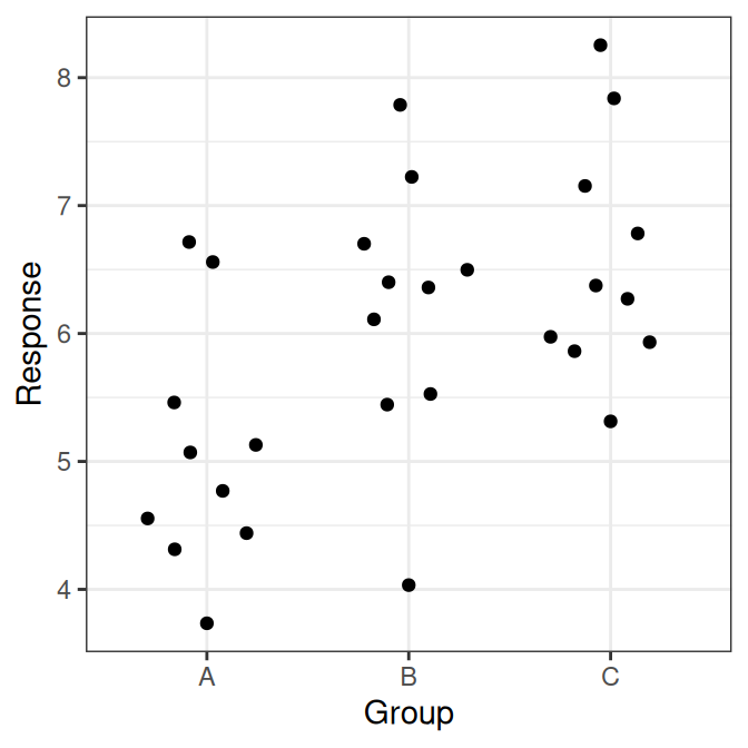
In R, a one-way ANOVA can be fitted using aov, and post hoc comparisons can be performed using TukeyHSD:
            Df Sum Sq Mean Sq F value  Pr(>F)
group        2  12.24   6.122   6.435 0.00518 **
Residuals   27  25.68   0.951
---
Signif. codes:  0 '***' 0.001 '**' 0.01 '*' 0.05 '.' 0.1 ' ' 1
Tukey multiple comparisons of means
95% family-wise confidence level
Fit: aov(formula = response ~ group, data = df)
$group
diff lwr upr p adj
B-A 1.1339963 0.05254072 2.215452 0.0384525
C-A 1.5008155 0.41935988 2.582271 0.0052283
C-B 0.3668192 -0.71463643 1.448275 0.6812485If the ANOVA test is not significant, post hoc pairwise comparisons are usually not performed.
If the assumptions of one-way ANOVA are not fulfilled, a rank-based alternative is the Kruskal–Wallis test. This test compares the groups using the ranks of the observations rather than the raw values.
The null hypothesis is that the mean ranks of the groups are the same. A significant Kruskal–Wallis test indicates that at least one group differs from the others, but like ANOVA, it does not show which groups differ.
In R, the Kruskal–Wallis test can be performed using the function kruskal.test.
    Kruskal-Wallis rank sum test

data:  response by group
Kruskal-Wallis chi-squared = 8.1858, df = 2, p-value = 0.01669