The visualization tutorial here is inspired from the NBIS workshop on Single-cell RNA-seq Analysis. The visualization tutorial here are part of the single-cell workshop as well.

1 Get data

In this tutorial, we will run all tutorials with a set of 8 PBMC 10x datasets from 4 covid-19 patients and 4 healthy controls, the samples have been subsampled to 1500 cells per sample. We can start by defining our paths.

path_covid <- "./data/covid/"
if (!dir.exists(path_covid)) dir.create(path_covid, recursive = T)

download.file("https://lu.box.com/shared/static/205zwfegtinm49yuelbvxawln6r3wyjd", destfile = file.path(path_covid, "seurat_covid_raw.rds"))
download.file("https://lu.box.com/shared/static/nf5eps2uus9qcjx0ml0n313p9a8r1vb7", destfile = file.path(path_covid, "seurat_covid_qc_dr_clst.rds"))

# If downloading via R terminal fails, you can download the images directly using the following links:
# seurat_covid_raw.rds: https://lu.box.com/s/205zwfegtinm49yuelbvxawln6r3wyjd
# seurat_covid_qc_dr_clst.rds: https://lu.box.com/s/nf5eps2uus9qcjx0ml0n313p9a8r1vb7

With data in place, now we can start loading libraries we will use in this tutorial.

suppressPackageStartupMessages({
    library(Seurat)
    library(Matrix)
    library(ggplot2)
    library(patchwork)
    library(dplyr)
    library(tidyverse)
})
covid_raw <- readRDS("./data/covid/seurat_covid_raw.rds")
covid_final <- readRDS("./data/covid/seurat_covid_qc_dr_clst.rds")

All the eight different datasets mentioned above are already merged into a single Seurat object. The two files you have downloaded are explained below:

seurat_covid_raw.rds: Contains all the data in raw format. There was no pre-processing of the data done here.
seurat_covid_qc_dr_clst.rds: In this file, the cells and the genes went through a different QC process, followed by Dimentionality Reduction and Clustering.

2 Raw data

Let us just take a look at the raw-data to start with. Here is how to take a look at the count matrix and the metadata for every cell.

# rna counts matrix
covid_raw[["RNA"]]$counts[1:10, 1:4] 

# metadata of the cells
head(covid_raw@meta.data, 10)

When you look at the metadata you can see the rownames are ids of each cell. Each of the column is explained below.

orig.ident: represents the patient id.
nCount_RNA: the total number of molecules detected within a cell
nFeature_RNA: the number of genes detected in each cell
type: If the sample is covid or control
percent_mito: Mitochondrial gene content in percent
percent_ribo: Ribosomal gene content in percent
percent_hb: Percentage haemoglobin genes
percent_plat: Percentage for some platelet markers

Thee values are pre-calculated to help assist with the visualization.

2.1 Plot QC

To plot the raw QC of the dataset, we will use the function VlnPlot(). This is a function from the Seurat package and it basically generates a ggplot2 object from the Seurat object. Violin plots are a different way of looking at boxplot.

feats <- c("nFeature_RNA", "nCount_RNA", "percent_mito", "percent_ribo", "percent_hb", "percent_plat")
VlnPlot(covid_raw, group.by = "orig.ident", split.by = "type", features = feats, pt.size = 0.1, ncol = 3)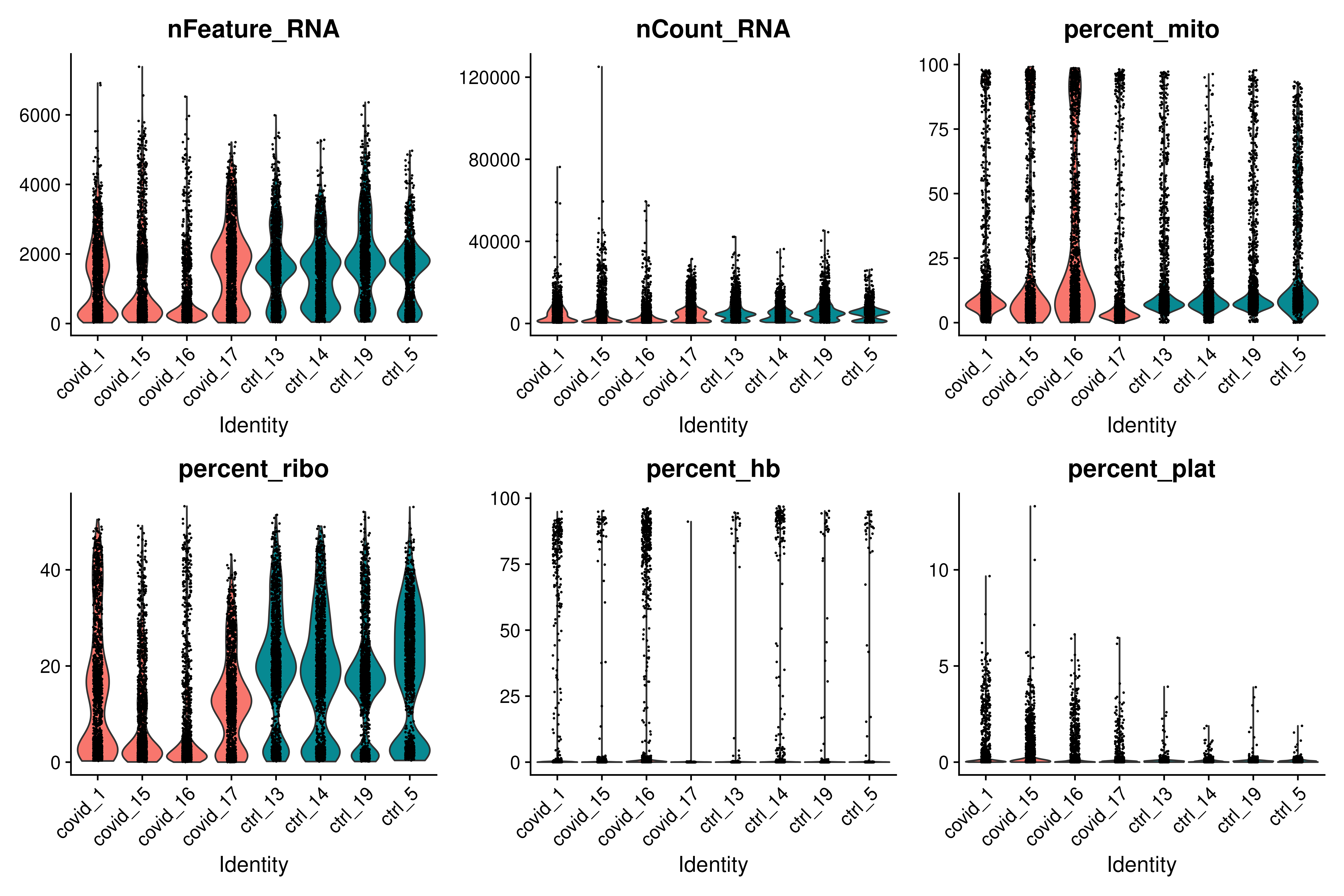

As you can see, there is quite some difference in quality for these samples, with for instance the covid_15 and covid_16 samples having cells with fewer detected genes and more mitochondrial content. As the ribosomal proteins are highly expressed they will make up a larger proportion of the transcriptional landscape when fewer of the lowly expressed genes are detected. We can also plot the different QC-measures as scatter plots.

FeatureScatter(covid_raw, "nCount_RNA", "nFeature_RNA", group.by = "orig.ident", pt.size = .5)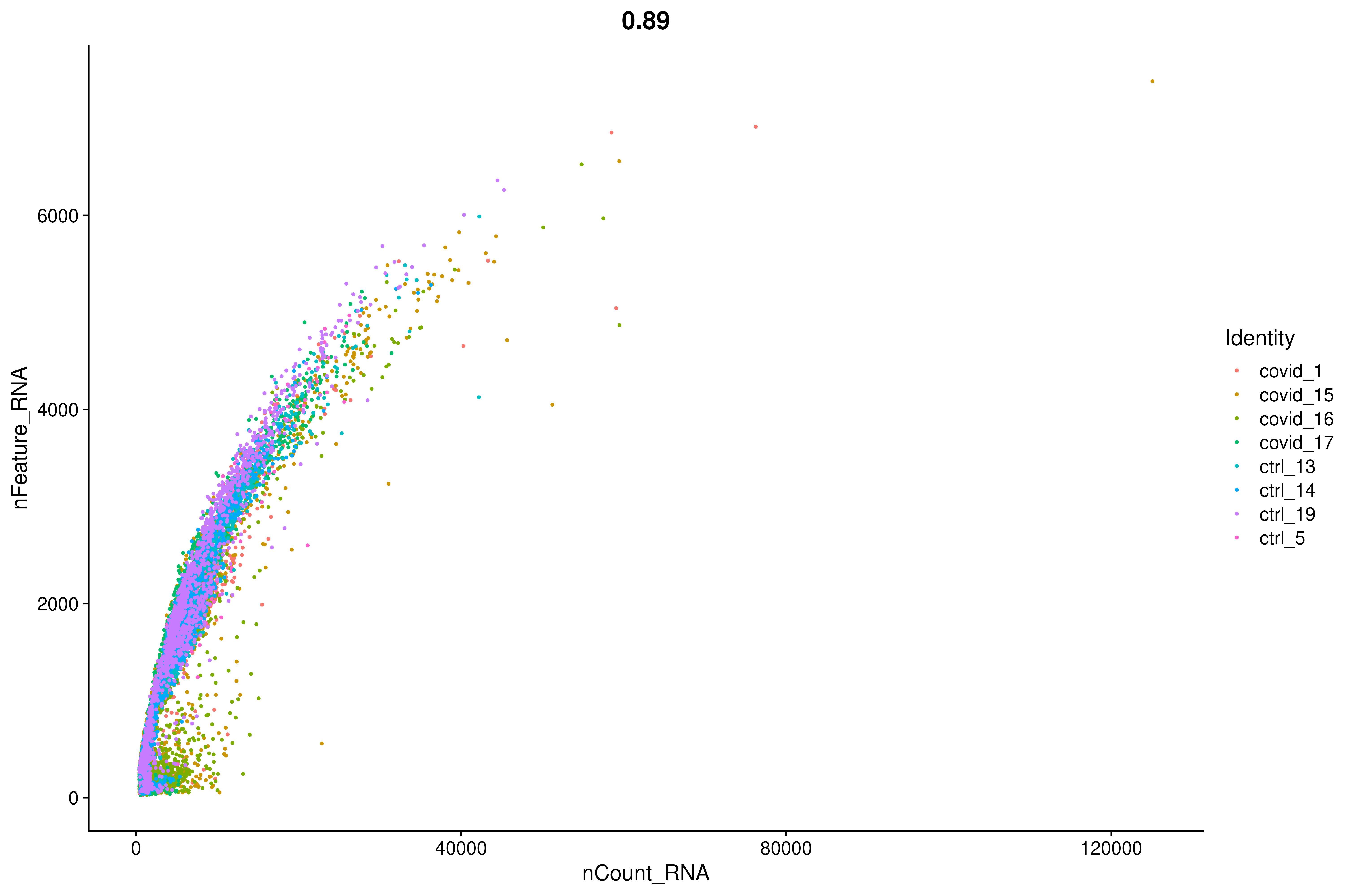

2.2 Plot Genes

Extremely high number of detected genes could indicate doublets. However, depending on the cell type composition in your sample, you may have cells with higher number of genes (and also higher counts) from one cell type. Additionally, we can also see which genes contribute the most to such reads. We can for instance plot the percentage of counts per gene.

# Compute the proportion of counts of each gene per cell
# Use sparse matrix operations, if your dataset is large, doing matrix divisions the regular way will take a very long time.

C <- covid_raw[["RNA"]]$counts
C@x <- C@x / rep.int(colSums(C), diff(C@p)) * 100
most_expressed <- order(Matrix::rowSums(C), decreasing = T)[20:1]

most_exp_long <- as.data.frame(t(C[most_expressed, ])) %>%
    rownames_to_column(var = "Cell") %>%
    gather(Gene, count, -Cell)

ggplot(most_exp_long) +
    geom_boxplot(aes(factor(Gene, levels = row.names(C[most_expressed, ])), count, fill = factor(Gene, levels = row.names(C[most_expressed, ])))) +
    coord_flip() +
    ylab("Percent counts per cell") +
    xlab(("")) +
    theme_classic() +
    theme(legend.position = "none")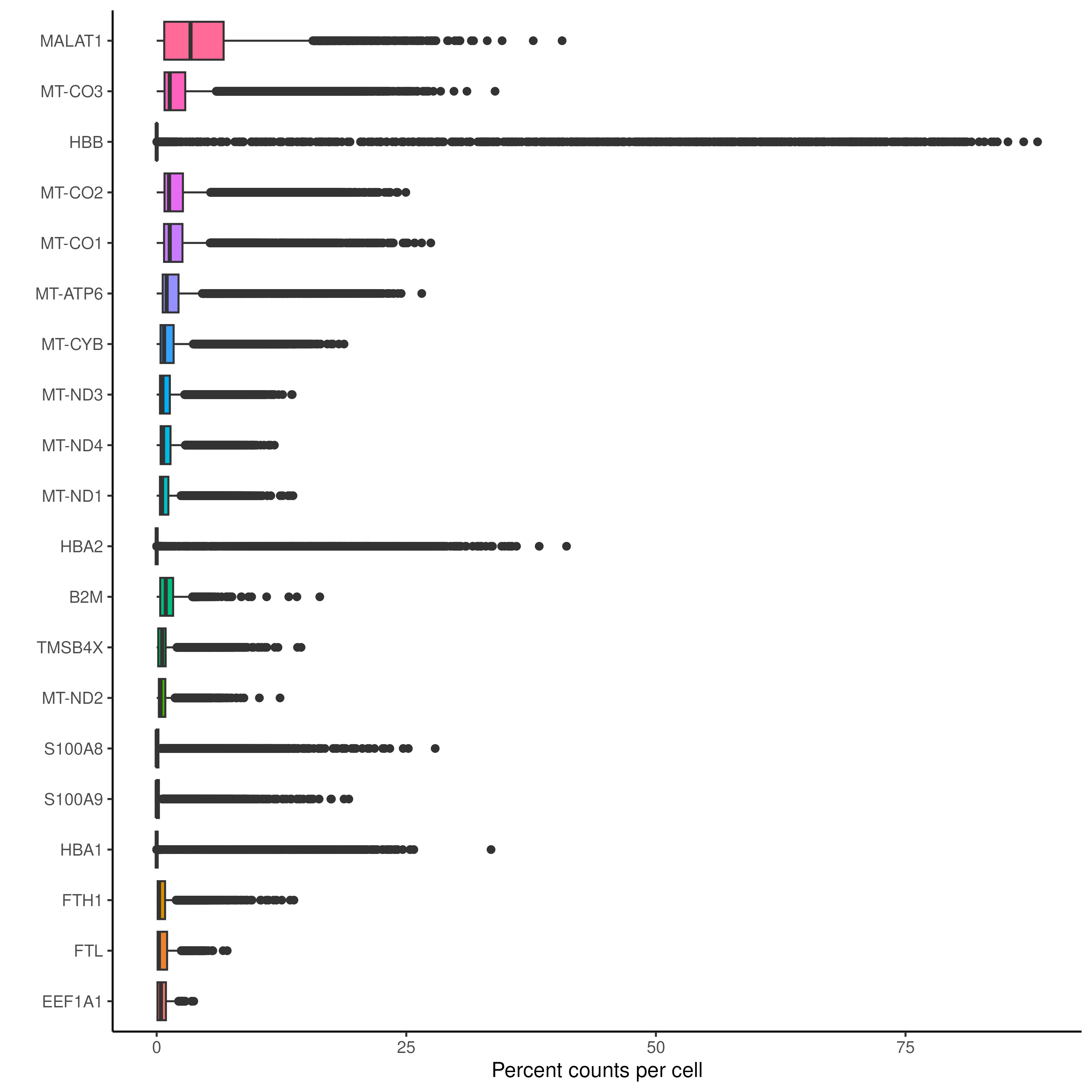

Note

The above plot and the code for the plot is very loaded. It is advised to go through them a bit carefully.

As you can see from the plot, the genes like MALAT1, the haemoglobin gene HBB and HBA2 and the several mitochondrial genes MT- are technical artifacts that needs to be removed.

3 Post filtration

There has been multiple filters applied to the above Seurat object containing raw data. Few of those are mentioned below:

cells with nFeature_RNA > 200
features with rowSums(covid_raw[["RNA"]]$counts) > 3
doublet prediction was applied for the cells and the doublets were removed.
MALAT1, HB and MT- genes were removed.

The filtered data is available in covid_final.

feats <- c("nFeature_RNA", "nCount_RNA", "percent_mito", "percent_ribo", "percent_hb", "percent_plat")
VlnPlot(covid_final, group.by = "orig.ident", split.by = "type", features = feats, pt.size = 0.1, ncol = 3)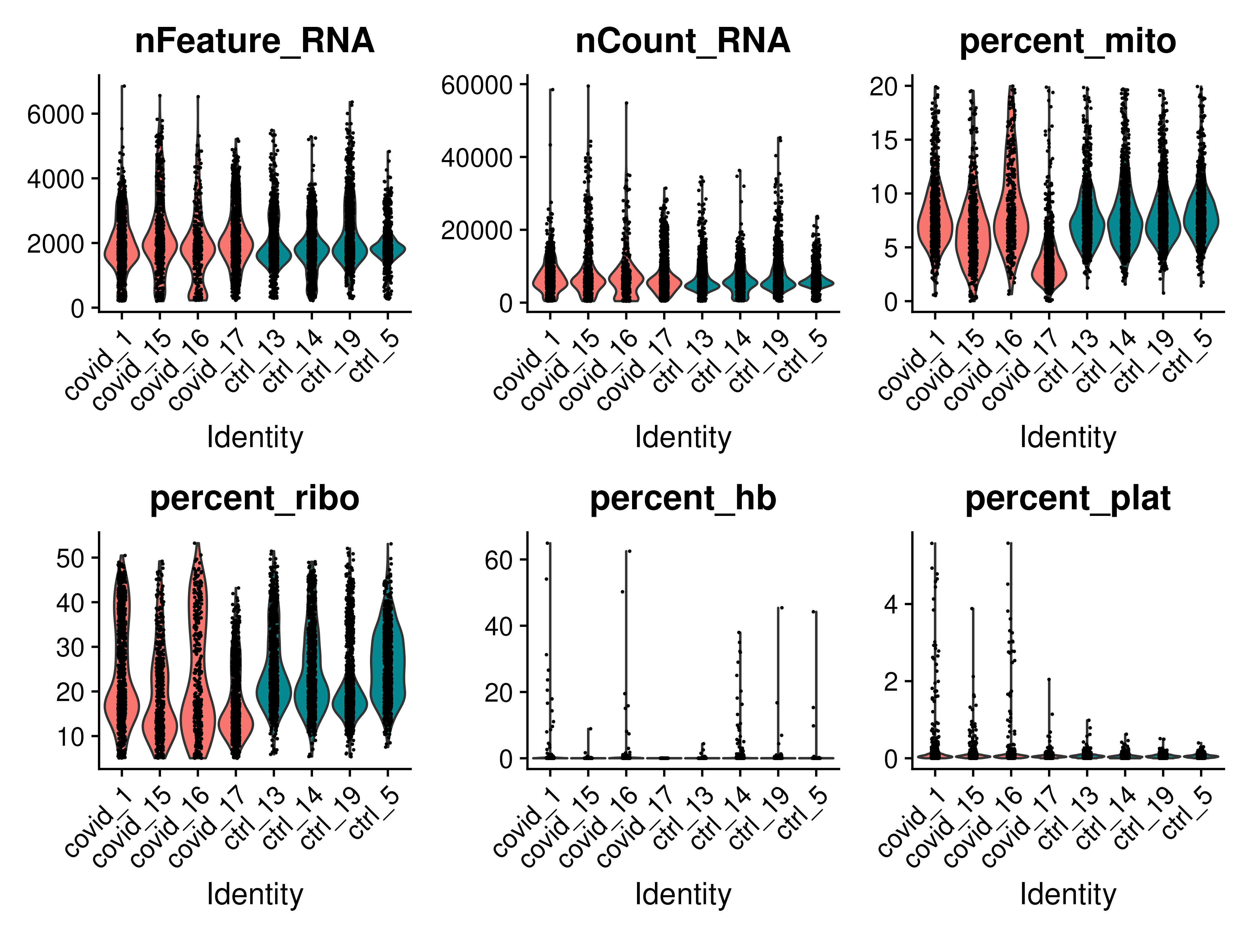

We could also test the scatter plot to see how the nCount_RNA and nFeature_RNA are related in this filtered data compared to the raw data.

FeatureScatter(covid_final, "nCount_RNA", "nFeature_RNA", group.by = "orig.ident", pt.size = .5)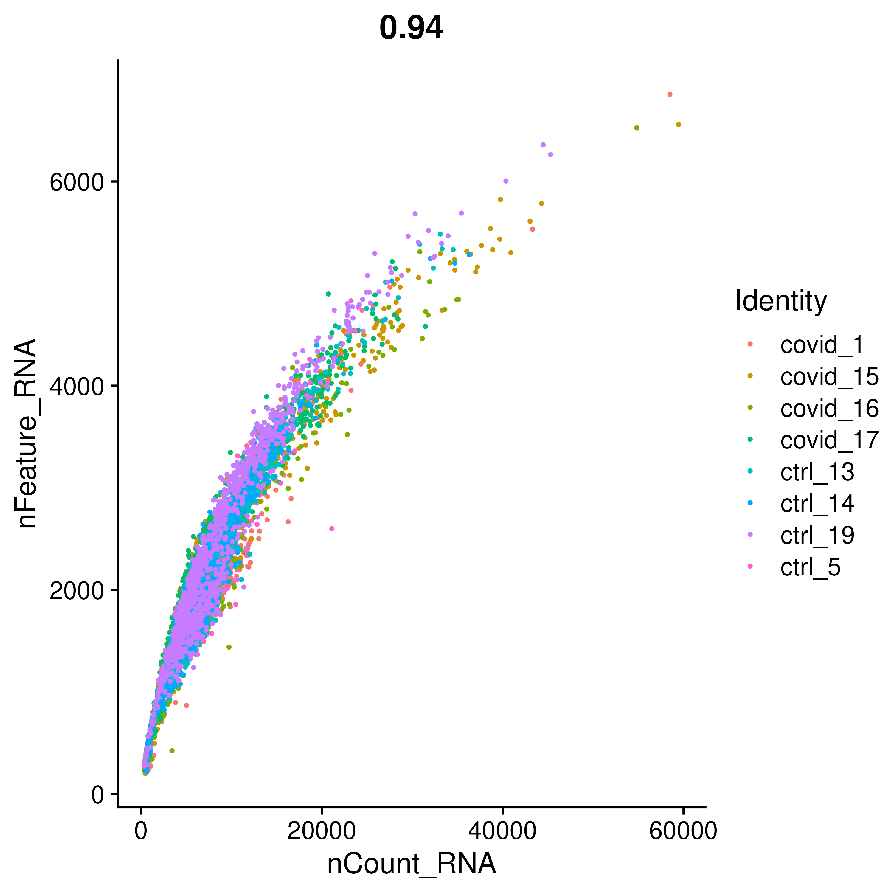

3.1 Sample Sex

When working with human or animal samples, you should ideally constrain your experiments to a single sex to avoid including sex bias in the conclusions. However this may not always be possible. By looking at reads from chromosomeY (males) and XIST (X-inactive specific transcript) expression (mainly female) it is quite easy to determine per sample which sex it is. It can also be a good way to detect if there has been any mislabelling in which case, the sample metadata sex does not agree with the computational predictions.

For your convenience, the percentage of ChrY genes were calculated in each cell. These are present in the covid_final object. We can sanity check our samples by plotting both scatter plots and violin plots.

FeatureScatter(covid_final, feature1 = "XIST", feature2 = "pct_chrY", group.by = "orig.ident", pt.size = .5)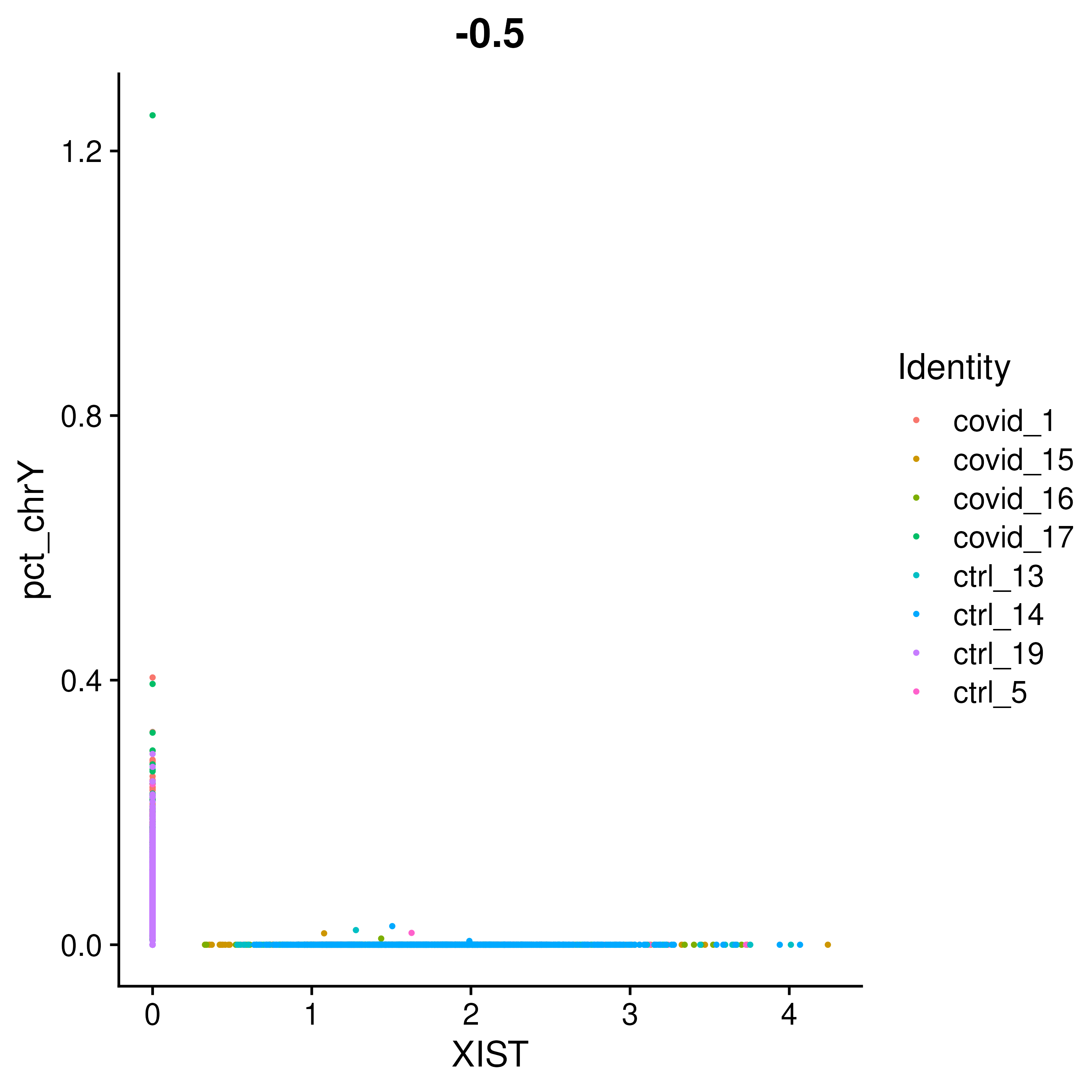

As you can see, the samples are clearly on either side, even if some cells do not have detection of either. Now let us plot this as violins to see which exact patients are Male and Female.

VlnPlot(covid_final, group.by = "orig.ident", split.by = "type", features = c("XIST", "pct_chrY"))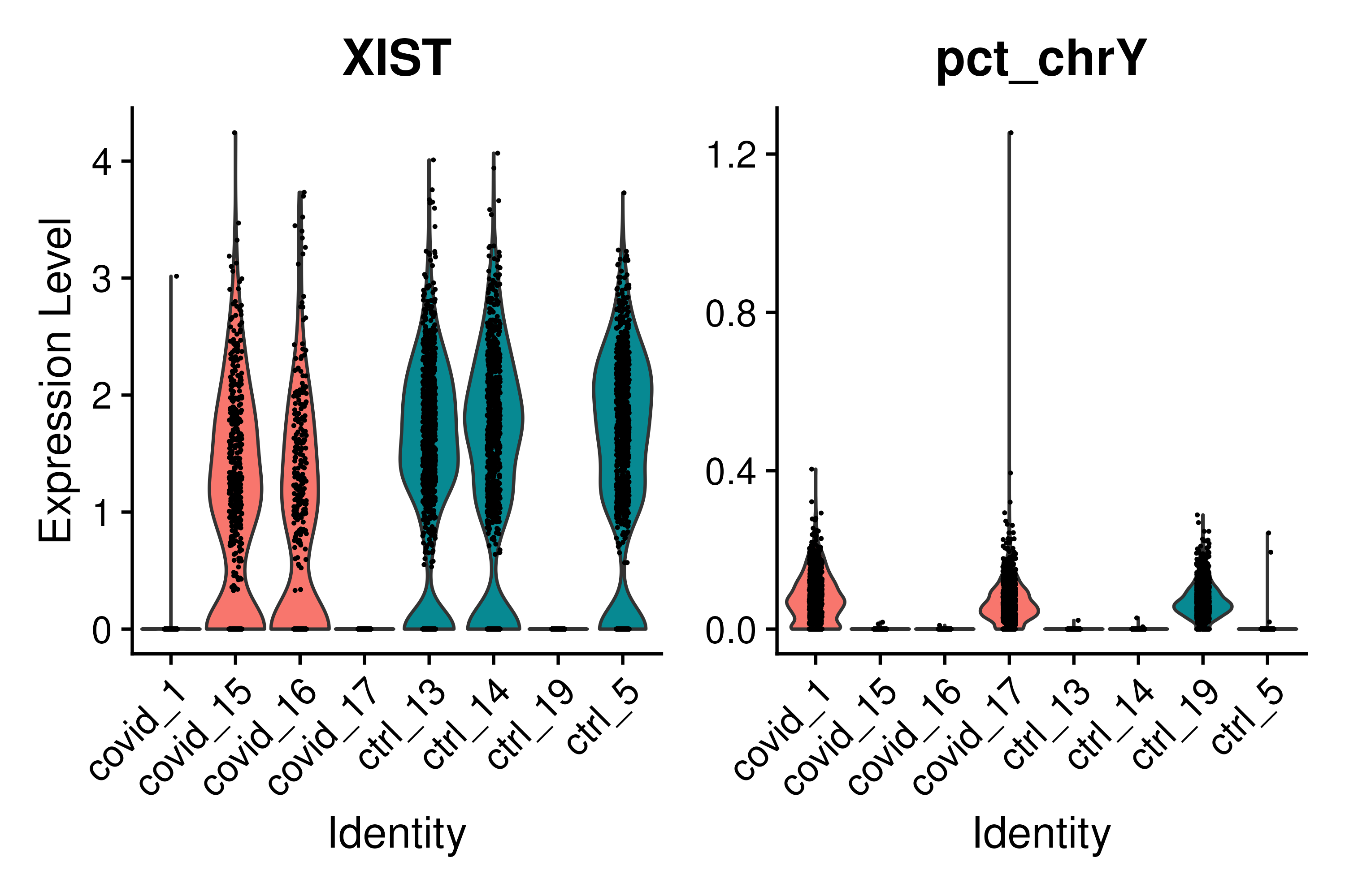

You can clearly tell from the above image that the samples covid_1, covid_17 and ctrl_19 are Male and the rest are Female. ## Cell cycle state

The cell cycle state of each was determined using CellCycleScoring() function. Cell cycle scoring adds three slots in the metadata, a score for S phase, a score for G2M phase and the predicted cell cycle phase.

VlnPlot(covid_final, features = c("S.Score", "G2M.Score"), group.by = "orig.ident", ncol = 2, pt.size = .1)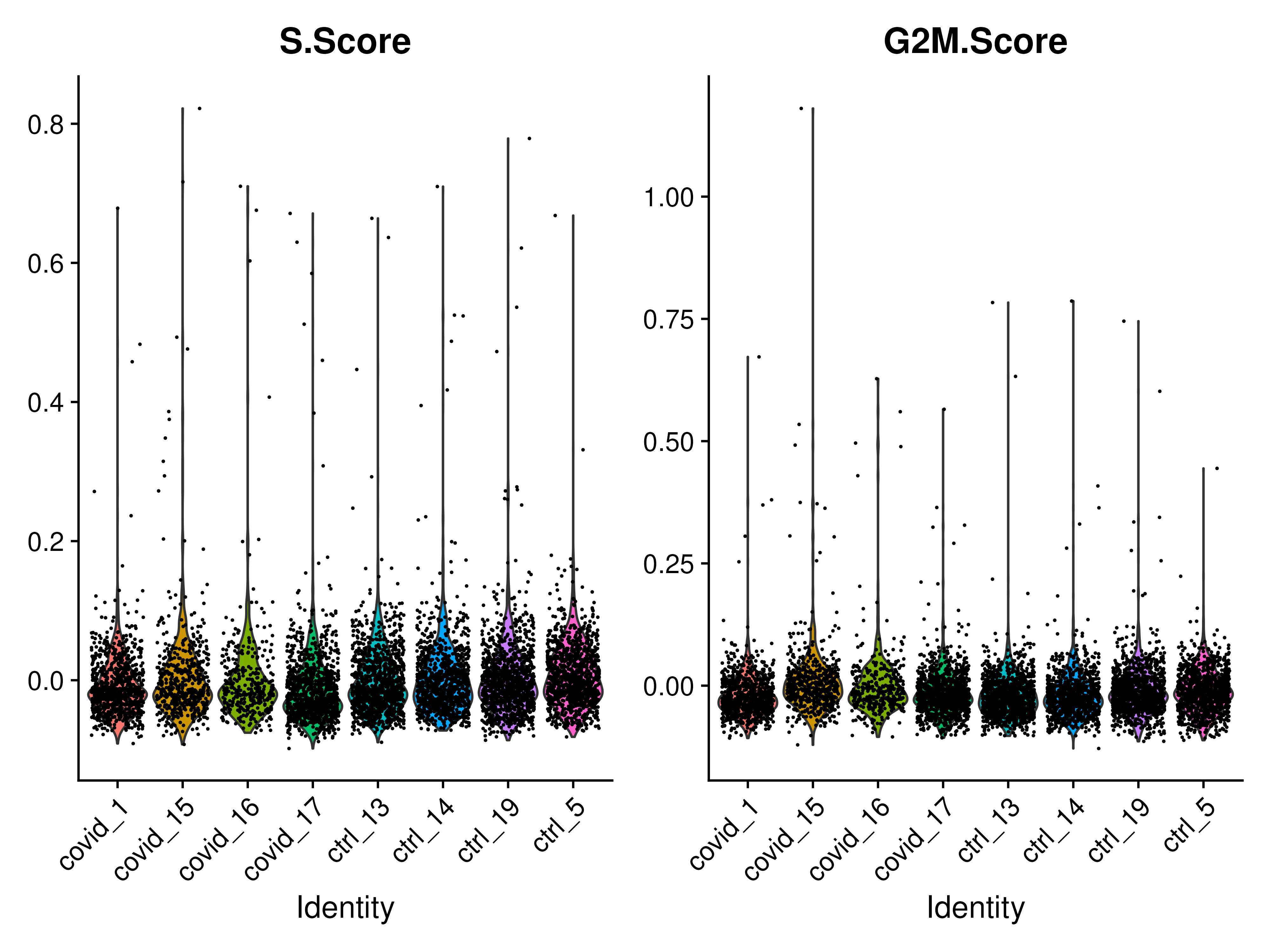

In this case it looks like we only have a few cycling cells in these datasets. We can also use the scatter plot and the prediction cell cycle phase.

FeatureScatter(covid_final, "S.Score", "G2M.Score", group.by = "Phase")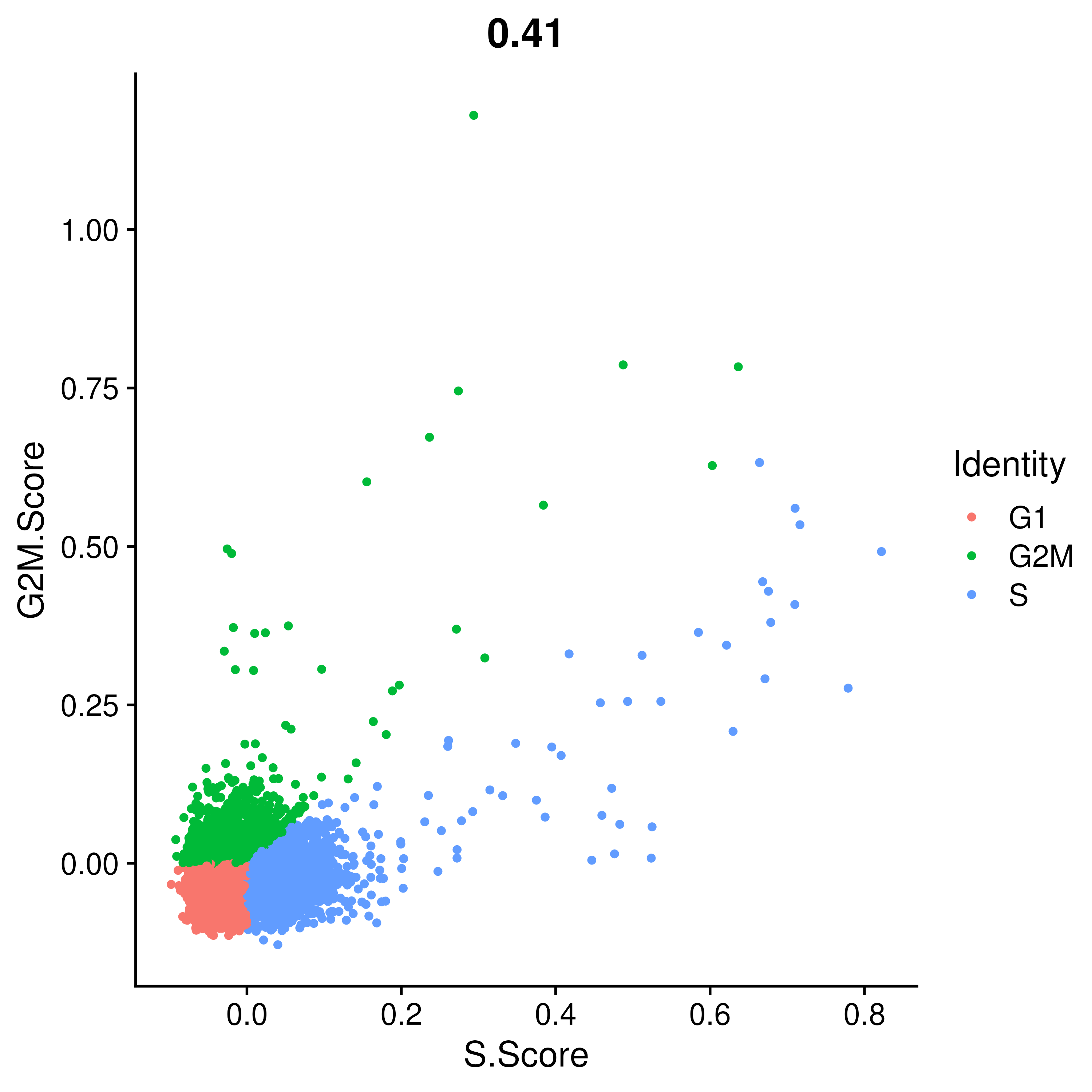

These are all the QC checks one usually does on a single-cell analysis. Now, let us also compare the number of cells present from each patient

> table(covid_raw$orig.ident)

 covid_1 covid_15 covid_16 covid_17  ctrl_13  ctrl_14  ctrl_19   ctrl_5 
    1500     1500     1500     1500     1500     1500     1500     1500 

> table(covid_final$orig.ident)

 covid_1 covid_15 covid_16 covid_17  ctrl_13  ctrl_14  ctrl_19   ctrl_5 
     875      549      357     1057     1126      996     1141     1033

4 Dimentionality Reduction

Usually with single-cell data, one needs to define which features/genes are important in the dataset to distinguish cell types. For this purpose, one needs to find genes that are highly variable across cells, which in turn will also provide a good separation of the cell clusters. We can usually visualize this by following:

suppressWarnings(suppressMessages(covid_final <- FindVariableFeatures(covid_final, selection.method = "vst", nfeatures = 2000, verbose = FALSE, assay = "RNA")))
top20 <- head(VariableFeatures(covid_final), 20)

LabelPoints(plot = VariableFeaturePlot(covid_final), points = top20, repel = TRUE)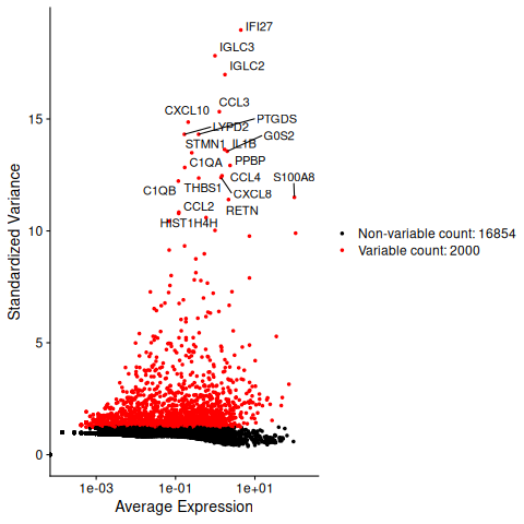

4.1 PCA

Now let us look into plotting PCA plots of this expression data. The object covid_final already has the data scaled with Z-score normalization in combination with regression to remove any unwanted sources of variation from the dataset, such as cell cycle, sequencing depth, percent mitochondria etc. PCA object was generated and stored in covid_final using the function RunPCA(). Below is how you would visualize the plots, for the sake of comparisons, 3 different PCA plots with the first six components are plotted:

wrap_plots(
    DimPlot(covid_final, reduction = "pca", group.by = "orig.ident", dims = 1:2),
    DimPlot(covid_final, reduction = "pca", group.by = "orig.ident", dims = 3:4),
    DimPlot(covid_final, reduction = "pca", group.by = "orig.ident", dims = 5:6),
    ncol = 3
) + plot_layout(guides = "collect")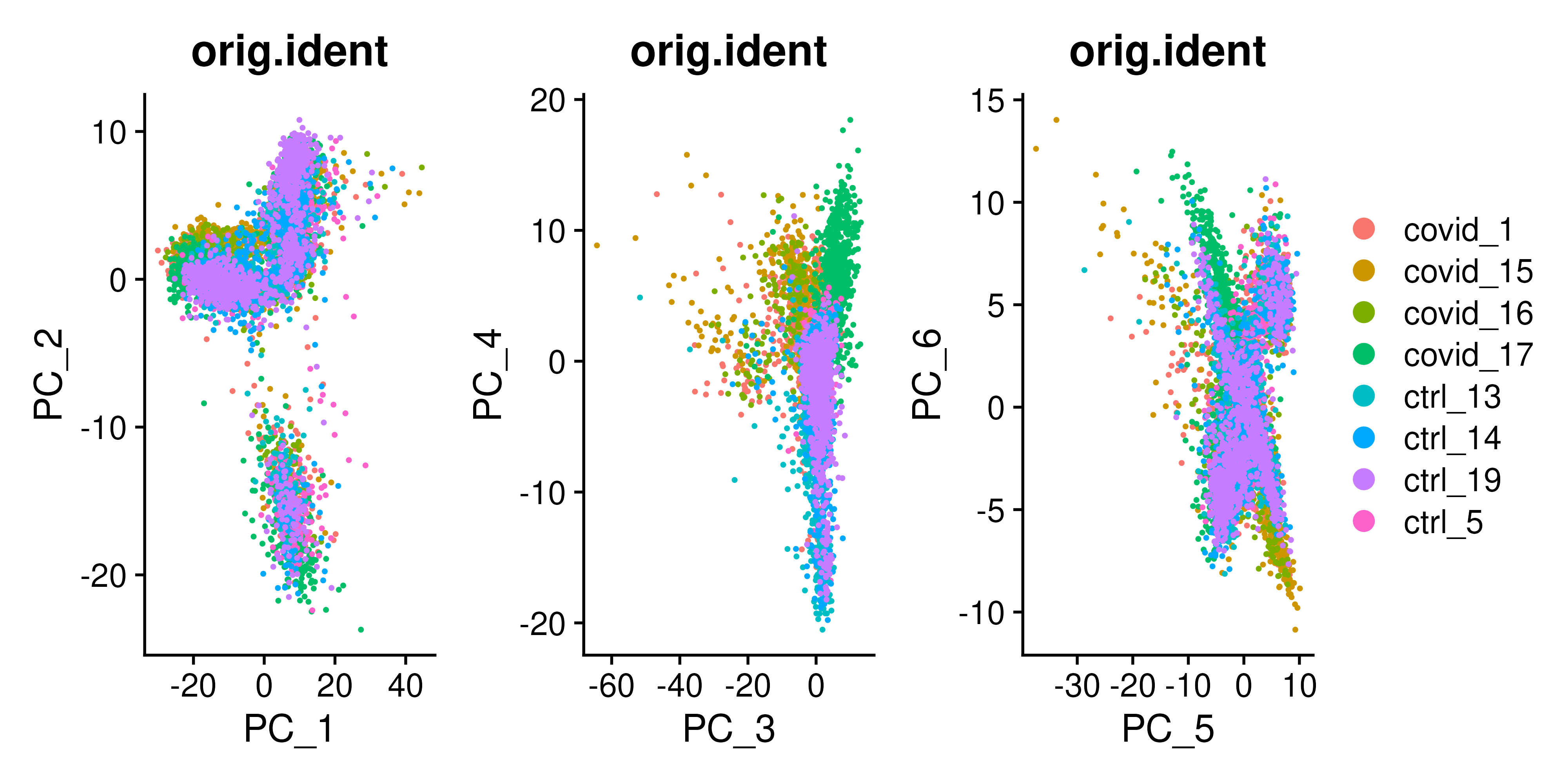

To identify which genes (Seurat) contribute the most to each PC, one can retrieve the loading matrix information.

VizDimLoadings(covid_final, dims = 1:5, reduction = "pca", ncol = 5, balanced = T)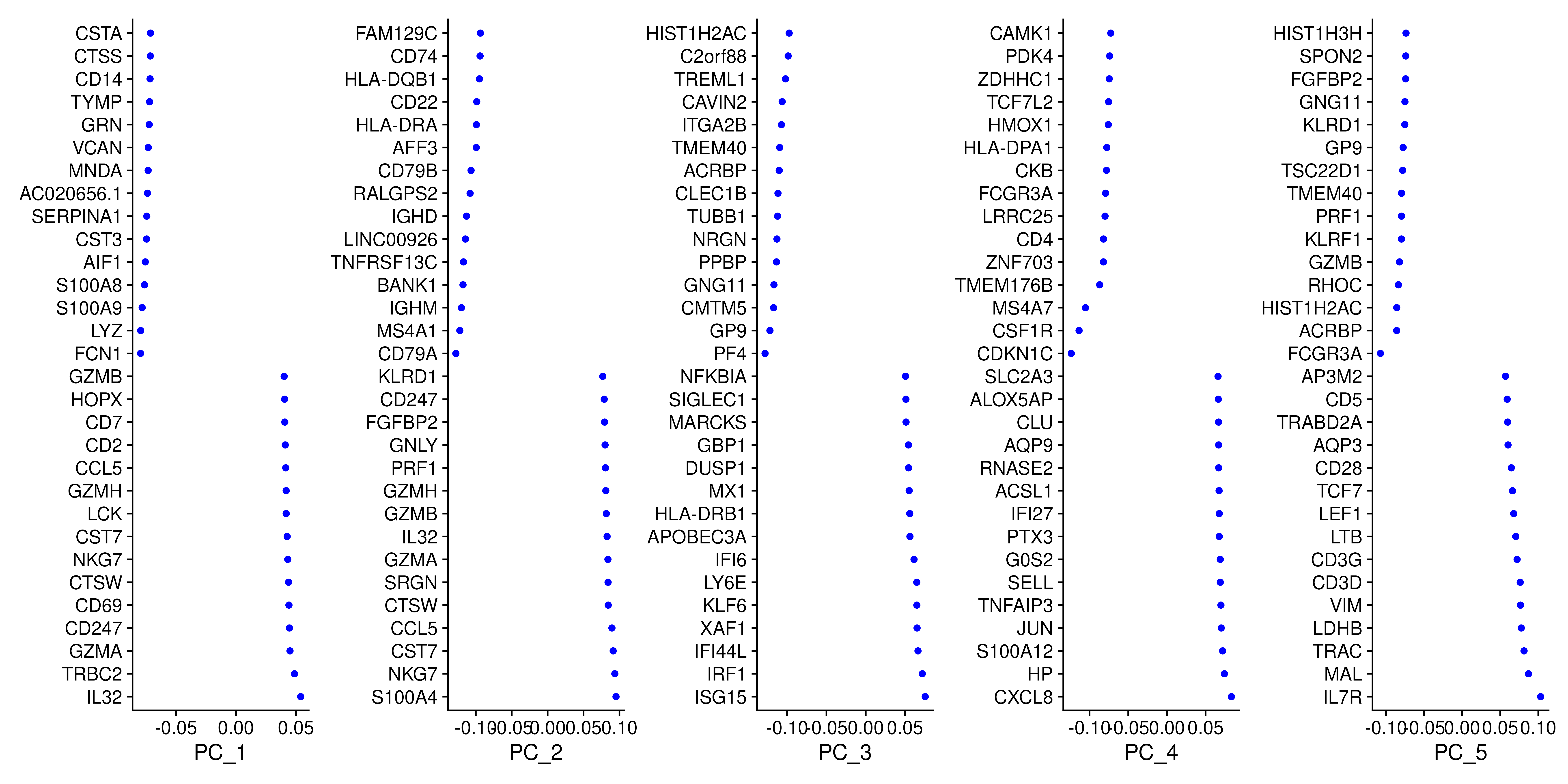

With the scater package we can check how different metadata variables contribute to each PCs. This can be important to look at to understand different biases you may have in your data.

Warning

Unfortunately we don’t have this package included in the list of R packages to be installed for this course. But, if you would really like to try, you can try to install it and run the following command. The example plot from the code is shown below.

scater::plotExplanatoryPCs(as.SingleCellExperiment(covid_final), nvars_to_plot = 15, npcs_to_plot = 20)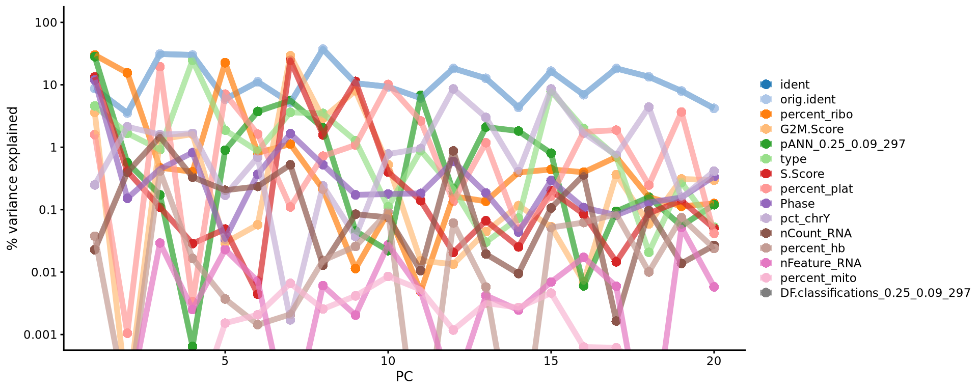

4.2 tSNE

tSNE is one of the main dimentionality reduction methods (non-linear) used for single-cell data and it is generated by using RunTSNE() function on the seurat object. We plot the tSNE scatterplot colored by dataset. We can clearly see the effect of batches present in the dataset.

DimPlot(covid_final, reduction = "tsne", group.by = "orig.ident")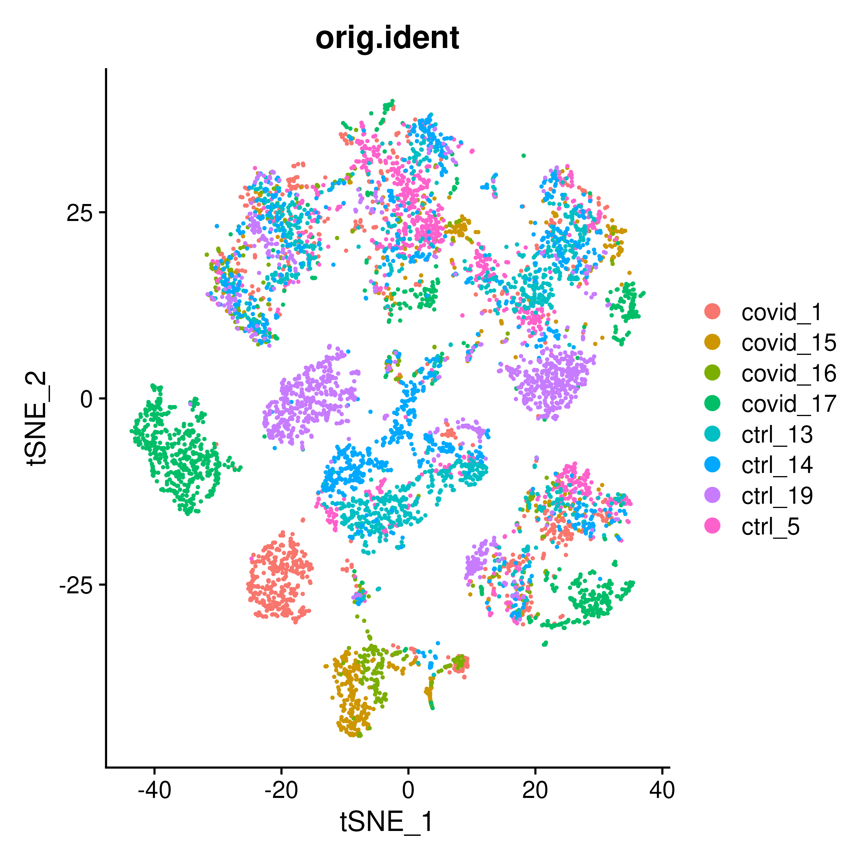

4.3 UMAP

Similar to tSNE, UMAP is an another well-known dimentionality reduction methods used with single-cell data. This is generated with the function RunUMAP(). Both tSNE and UMAP are usually generated from the PCA components. By default, RunUMAP only generates 2 UMAP components, but you can change this with the parameter n.components to have more more UMAP components.

covid_final has the following reductions stored in the object: - pca: PCA with 50 components built on scaled counts data - umap: UMAP with 2 components built on 30 PCA components - tsne: tSNE with 2 components built on 30 PCA components - UMAP10_on_PCA: UMAP with 10 components built on 30 PCA components - UMAP_on_ScaleData: UMAP with 2 components built on scaled counts data

wrap_plots(
    DimPlot(covid_final, reduction = "umap", group.by = "orig.ident") + ggplot2::ggtitle(label = "UMAP_on_PCA"),
    DimPlot(covid_final, reduction = "UMAP10_on_PCA", group.by = "orig.ident", dims = 1:2) + ggplot2::ggtitle(label = "UMAP10_on_PCA"),
    DimPlot(covid_final, reduction = "UMAP10_on_PCA", group.by = "orig.ident", dims = 3:4) + ggplot2::ggtitle(label = "UMAP10_on_PCA"),
    ncol = 3
) + plot_layout(guides = "collect")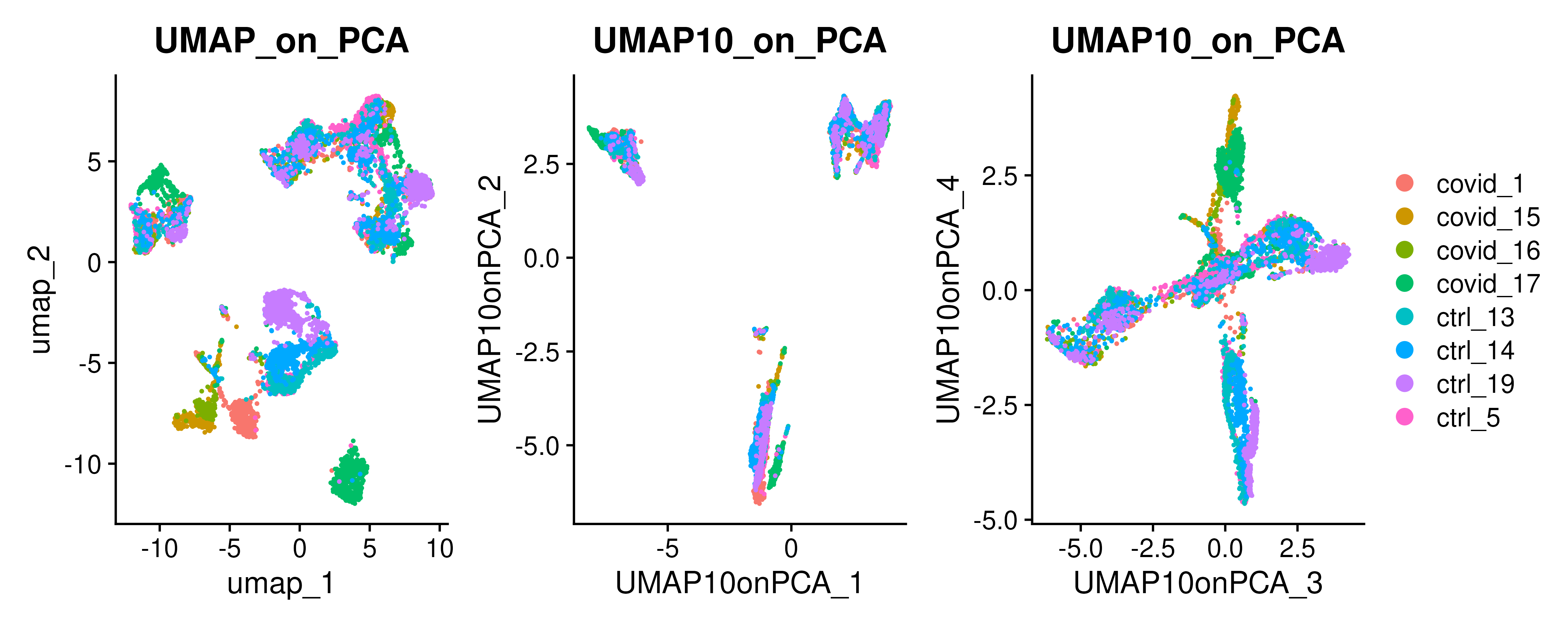

The above UMAP plots are colored per dataset. Although less distinct as in the tSNE, we still see quite an effect of the different batches in the data.

We can now plot PCA, UMAP and tSNE side by side for comparison.

wrap_plots(
    DimPlot(covid_final, reduction = "pca", group.by = "orig.ident") + ggplot2::ggtitle(label = "PCA"),
    DimPlot(covid_final, reduction = "tsne", group.by = "orig.ident") + ggplot2::ggtitle(label = "tSNE"),
    DimPlot(covid_final, reduction = "umap", group.by = "orig.ident") + ggplot2::ggtitle(label = "UMAP"),
    ncol = 3
) + plot_layout(guides = "collect")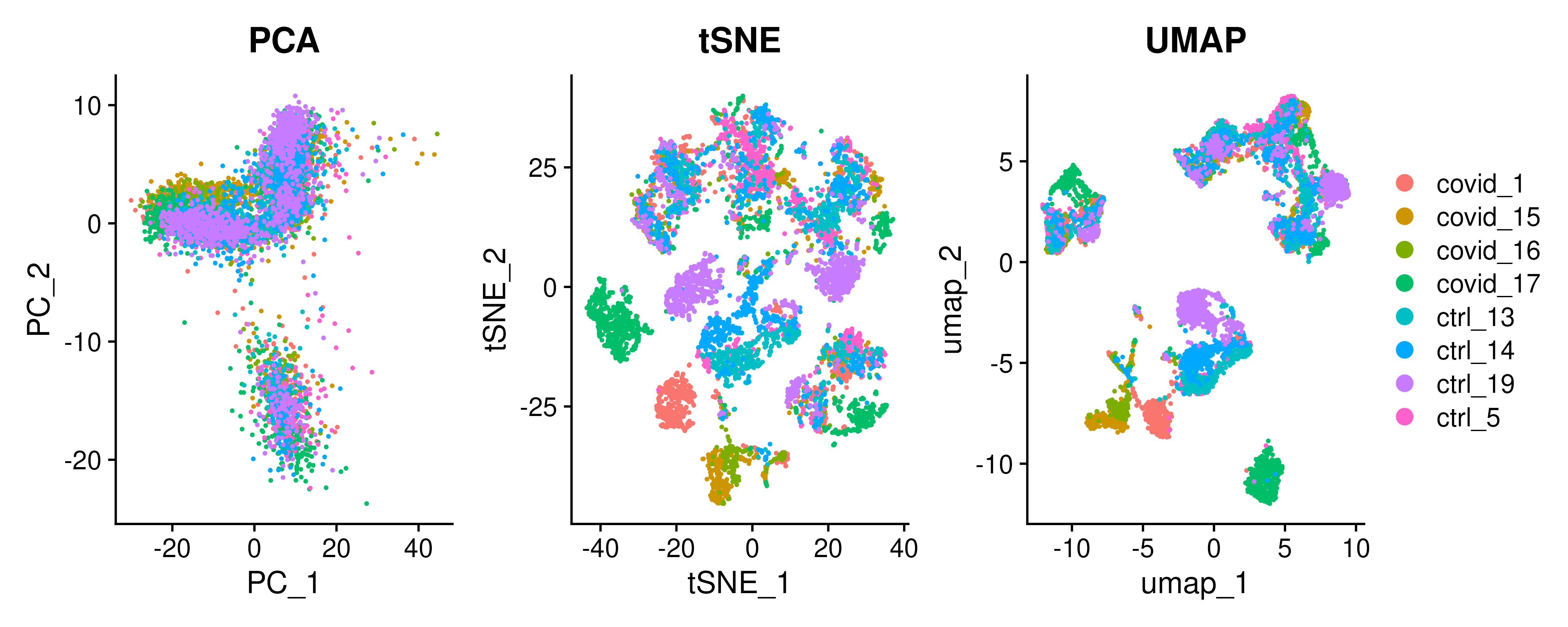

4.4 Features on DimPlot

It is possible to plot gene counts for different cell types onto the DimPlot embedding. Let us plot some marker genes.

myfeatures <- c("CD3E", "CD4", "CD8A", "NKG7", "GNLY", "MS4A1", "CD14", "LYZ", "MS4A7", "FCGR3A", "CST3", "FCER1A")
FeaturePlot(covid_final, reduction = "umap", dims = 1:2, features = myfeatures, ncol = 4, order = T)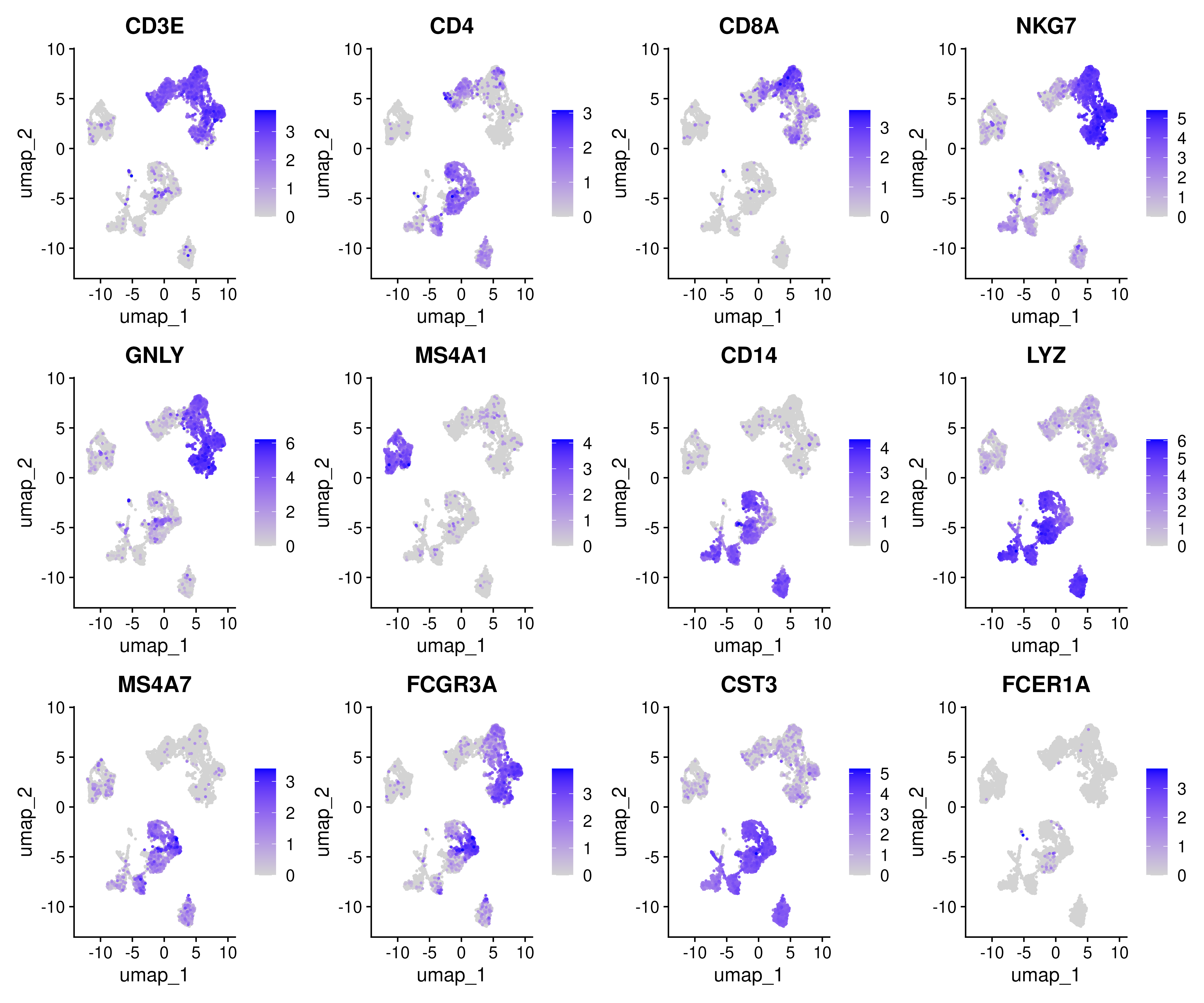

Similarly we can also plot metadata varibales onto the DimPlot embedding as well.

myfeatures <- c("nCount_RNA","nFeature_RNA", "percent_mito","percent_ribo","percent_hb","percent_plat")
FeaturePlot(covid_final, reduction = "umap", dims = 1:2, features = myfeatures, ncol = 3, order = T)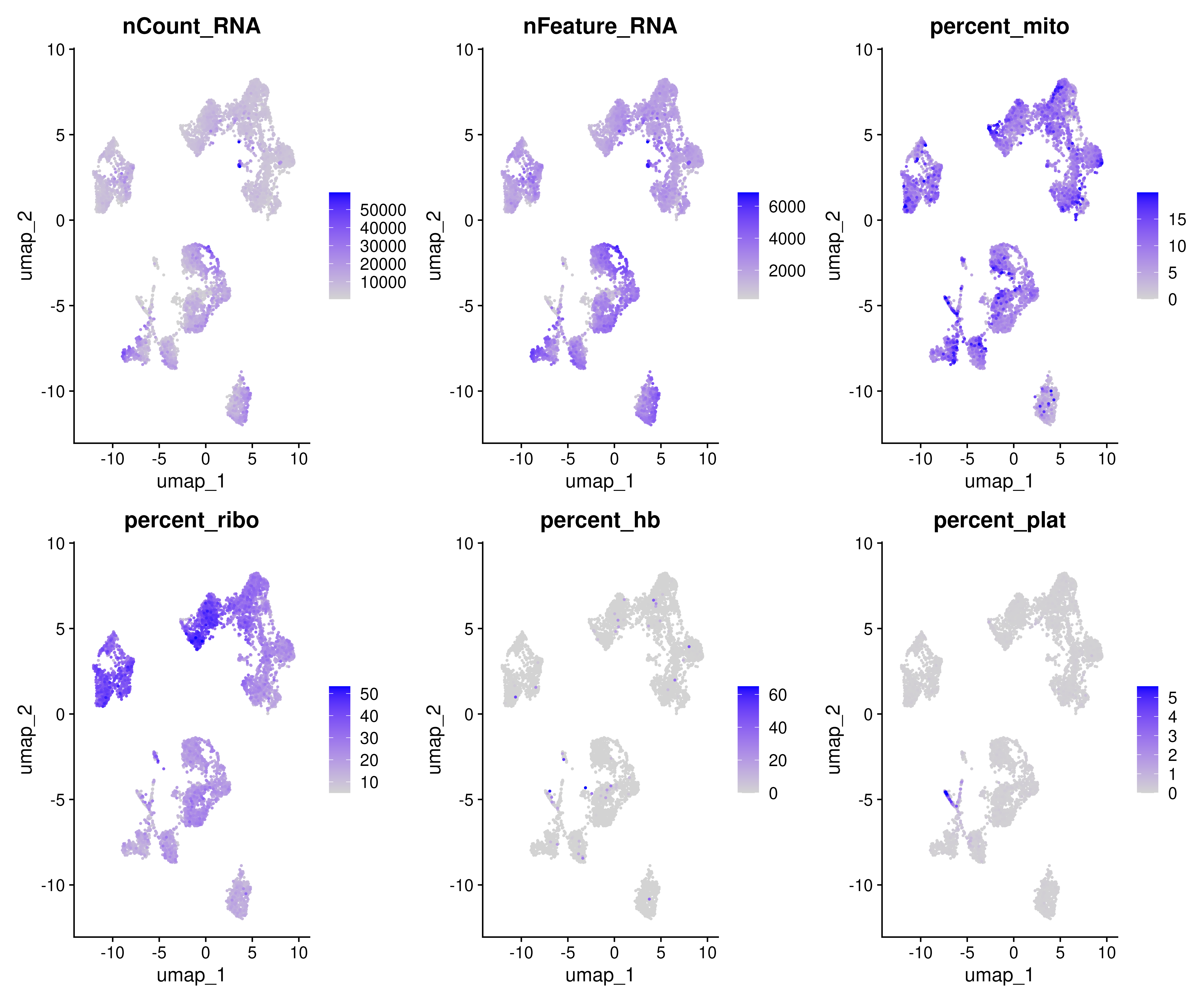

5 Clustering

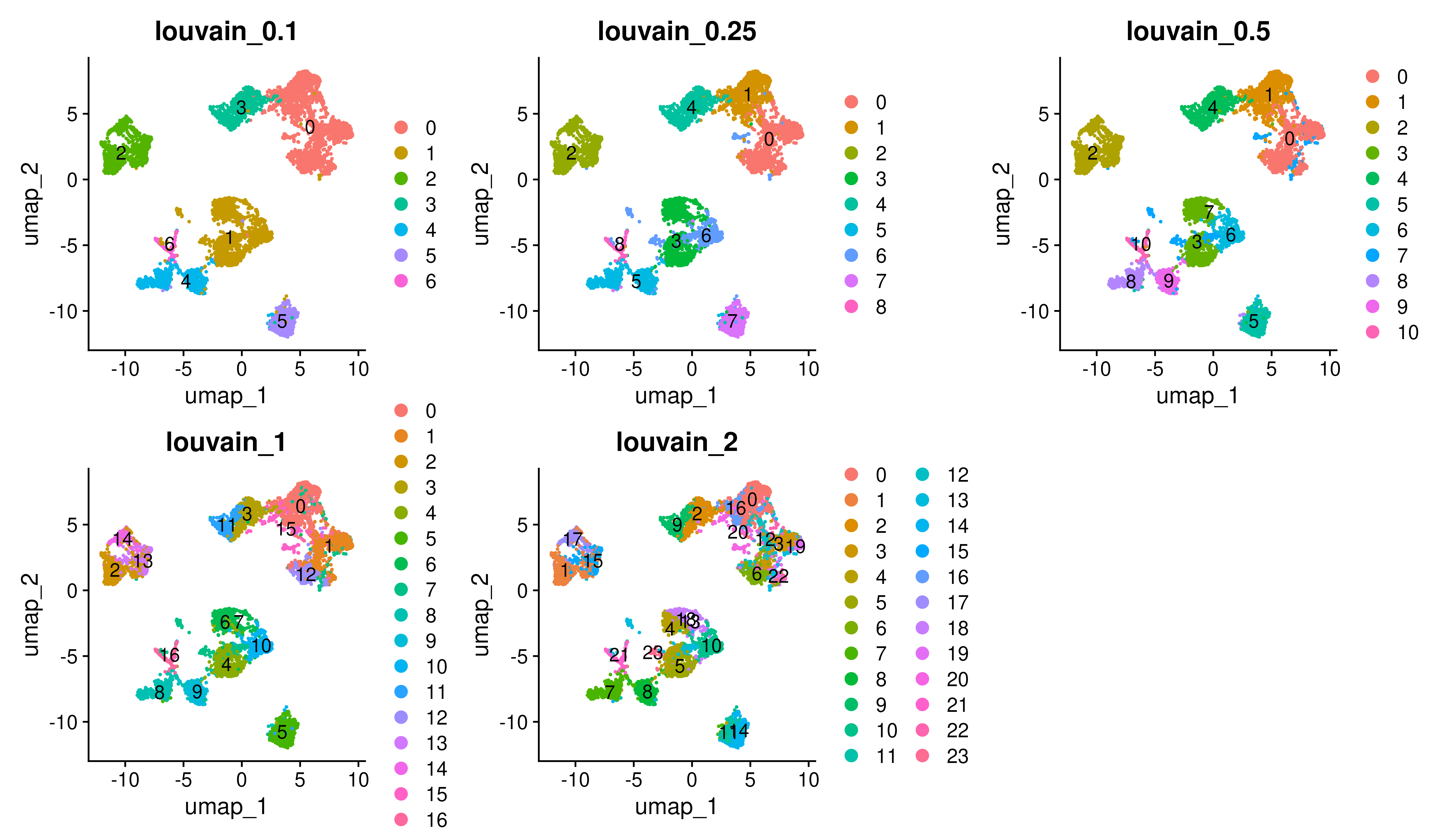
The object covid_final contains objects that the cells were clustered with louvain (algorithm 1) which is a graph based clustering with a few different resolutions.

wrap_plots(
    DimPlot(covid_final, reduction = "umap", group.by = "RNA_snn_res.0.1", label=T) + ggtitle("louvain_0.1"),
    DimPlot(covid_final, reduction = "umap", group.by = "RNA_snn_res.0.25", label=T) + ggtitle("louvain_0.25"),
    DimPlot(covid_final, reduction = "umap", group.by = "RNA_snn_res.0.5", label=T) + ggtitle("louvain_0.5"),
    DimPlot(covid_final, reduction = "umap", group.by = "RNA_snn_res.1", label=T) + ggtitle("louvain_1"),
    DimPlot(covid_final, reduction = "umap", group.by = "RNA_snn_res.2", label=T) + ggtitle("louvain_2"),
    ncol = 3
)

We can select one of our clustering methods and compare the proportion of samples across the clusters. Select the RNA_snn_res.0.5 and plot proportion of samples per cluster and also proportion covid vs ctrl.

p1 <- ggplot(covid_final@meta.data, aes(x = RNA_snn_res.0.5, fill = orig.ident)) +
    geom_bar(position = "fill")
p2 <- ggplot(covid_final@meta.data, aes(x = RNA_snn_res.0.5, fill = type)) +
    geom_bar(position = "fill")

p1 + p2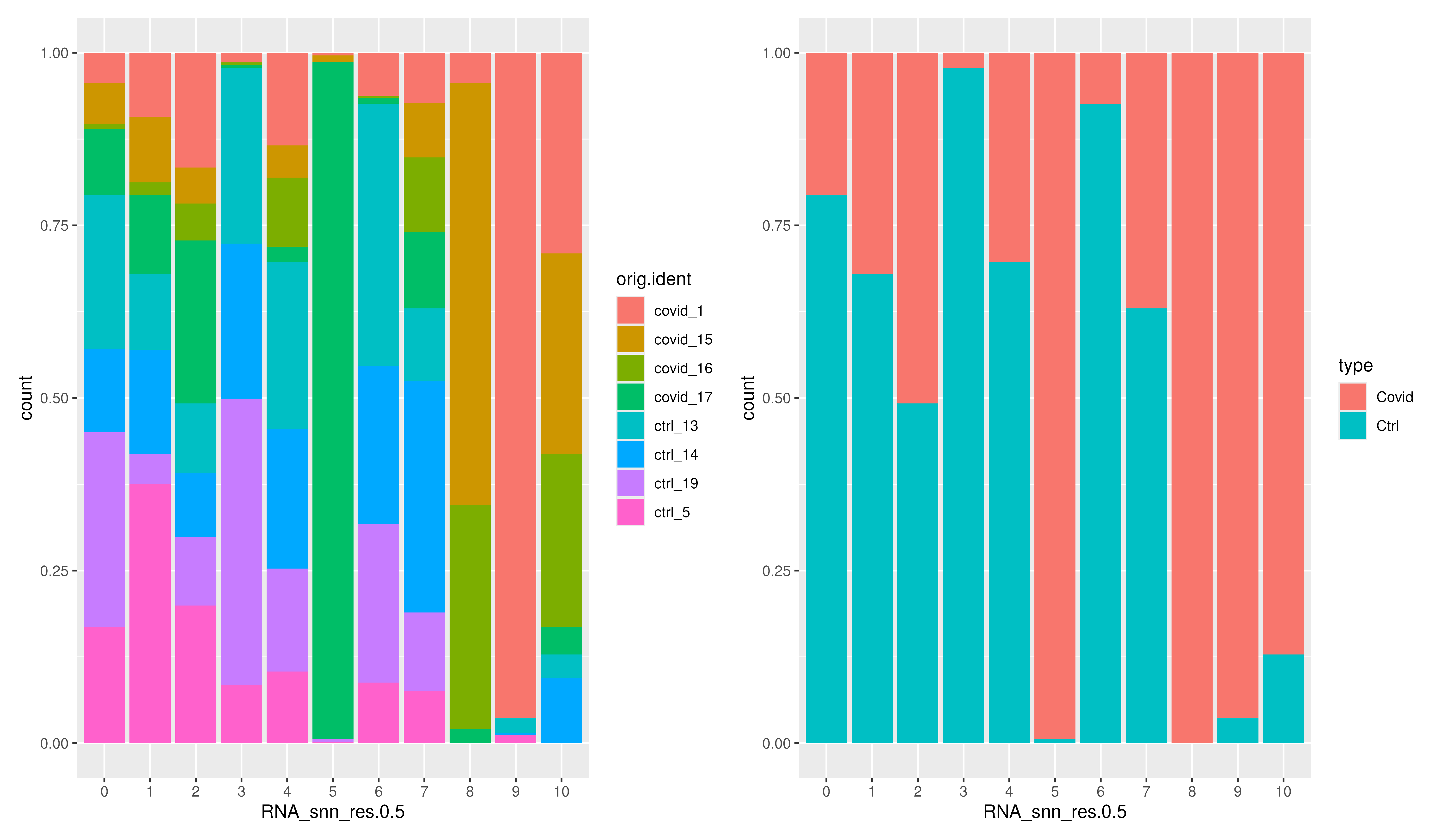

As you could see there are clearly biases with more cells from one sample in some clusters and also more covid/control cells in some of the clusters. Have look at clusters 3, 5, 8, 9 and 10.

Warning

This is an example of badly clustered data and it needs to be further pre-processes before down-stream analysis. Here we just focus on visualizing and also to show what kind of visualizations are important to keep track of the quality of the single-cell data. We will not discuss about how to pre-process, but you can checkout the workshop on single-cell analysis where we discuss the QC and downstream analysis in detail.

We can also plot the above plot in the other direction, the proportion of each cluster per sample.

ggplot(covid_final@meta.data, aes(x = orig.ident, fill = RNA_snn_res.0.5)) +
    geom_bar(position = "fill")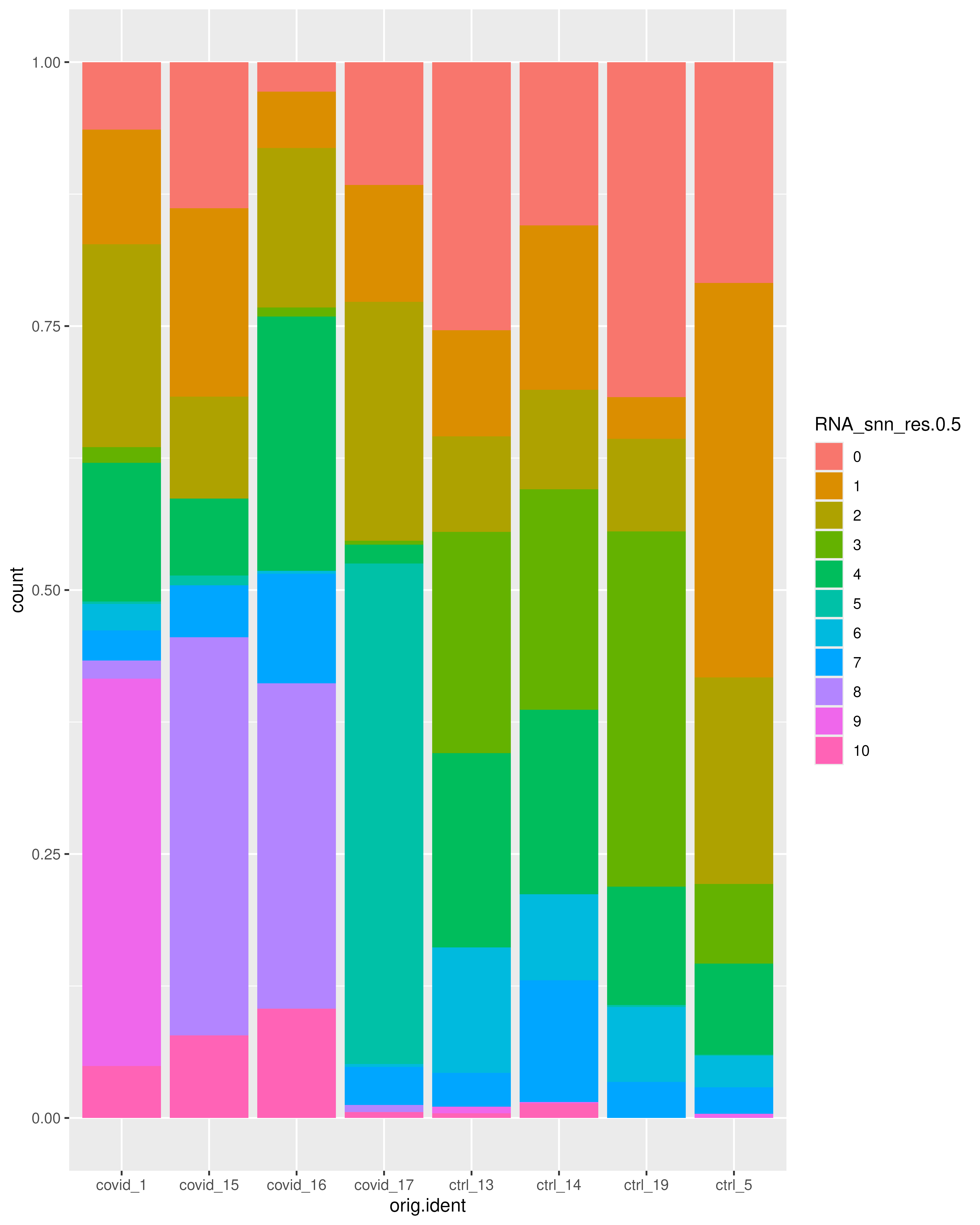

It is also good to check the distribution of other potential confounded variables that might affect the further analysis and their distribution among the clusters. For example:

VlnPlot(covid_final, group.by = "RNA_snn_res.0.5", features = c("nFeature_RNA", "percent_mito"))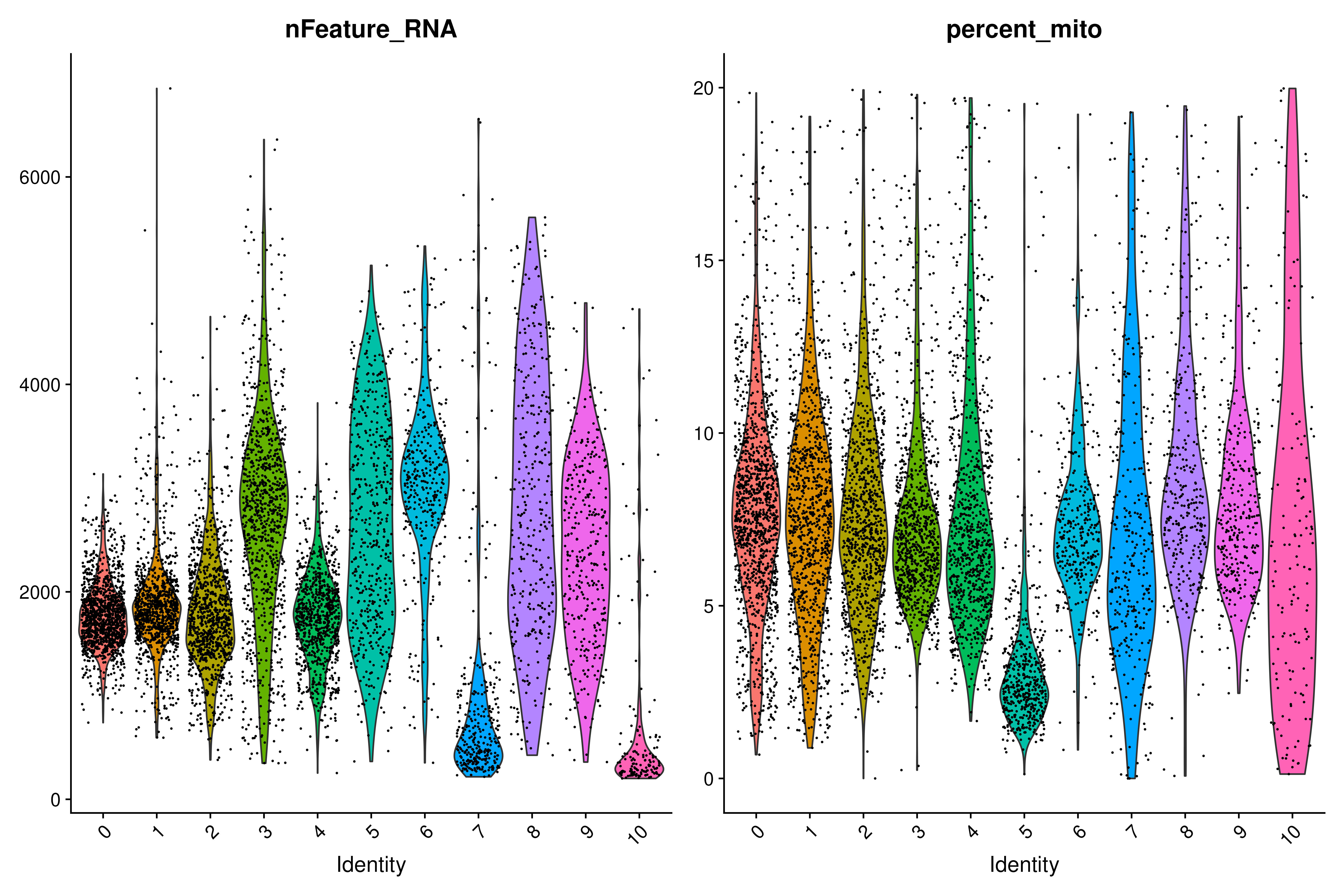

Once again, you can clearly see that there are biases in these clusters.

It is also good to check where your clusters are on a UMAP and how the marker gene expressions are correlating to the clusters. For example, lets find out where T-cell and NK-cell clusters are. We know that T-cells express CD3E, and the main subtypes are CD4 and CD8, while NK-cells express GNLY.

# check with the lowest resolution
p1 = DimPlot(alldata, reduction = "umap_cca", group.by = "RNA_snn_res.0.1", label = T) + ggtitle("louvain_0.1")
p2 = FeaturePlot(alldata, features = "CD3E", reduction = "umap_cca", order = T) 
p3 = FeaturePlot(alldata, features = "CD4", reduction = "umap_cca", order = T) 
p4 = FeaturePlot(alldata, features = "CD8A", reduction = "umap_cca", order = T) 
p5 = FeaturePlot(alldata, features = "GNLY", reduction = "umap_cca", order = T) 


wrap_plots(p1,p2,p3,p4,p5, ncol=3) + plot_layout(guides = "collect")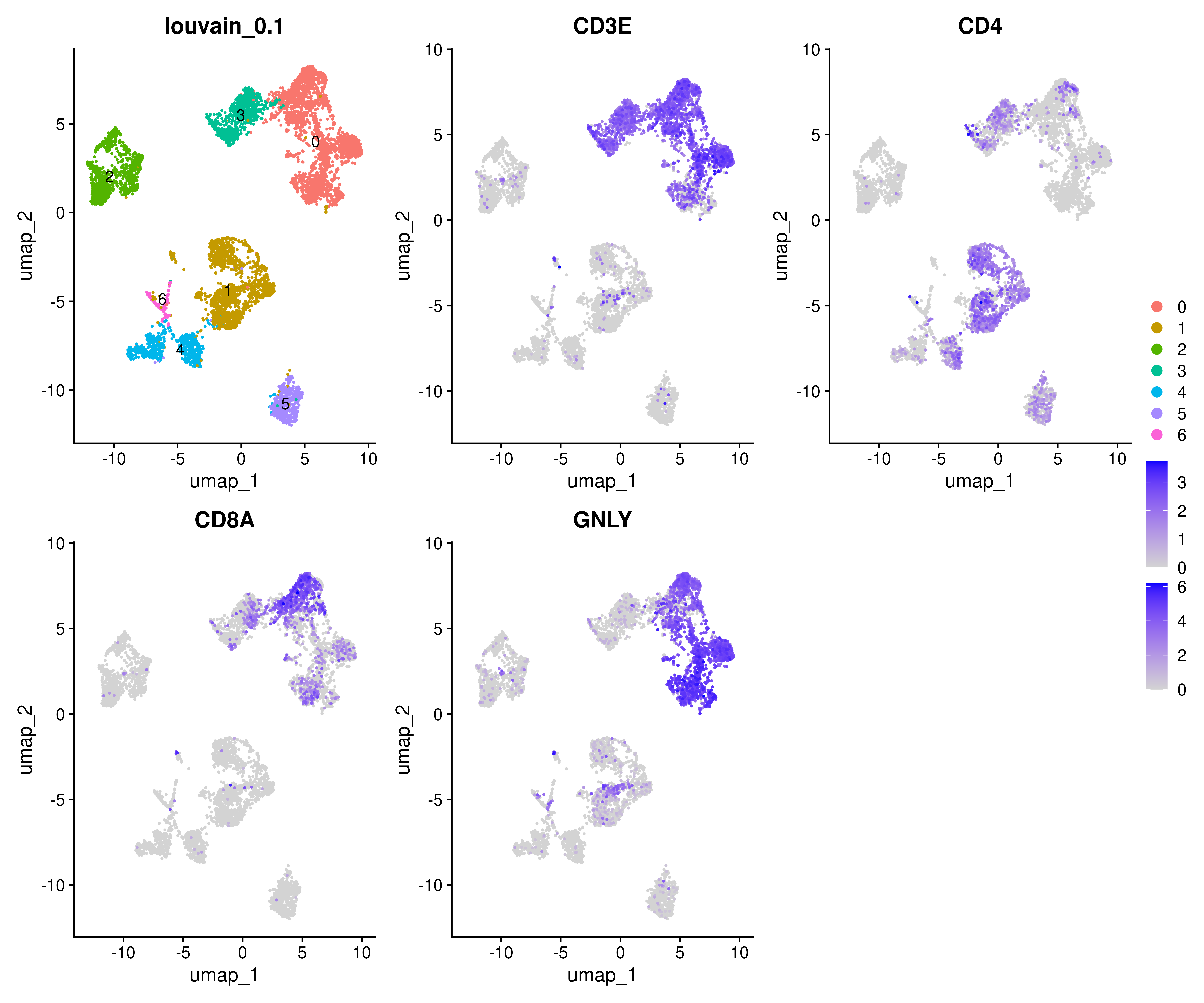

6 Differential Expression

Now let us run some differential expression and see how we can visualize them.

6.1 Across clusters

We will start with running a differential expression analysis between the different clusters. We will use the RNA_snn_res.0.5 clusters as an example for this.

sel.clust <- "RNA_snn_res.0.5"

covid_final <- SetIdent(covid_final, value = sel.clust)
table(covid_final@active.ident)

   0    1    2    3    4    5    6    7    8    9   10 
1283 1028 1012  926  858  511  353  343  339  333  148

We have 11 clusters in total and we will run the DGE analysis with the function FindAllMarkers from seurat that will run each of the clusters vs the rest. As you can see, there are some filtering criteria to remove genes that do not have certain log2FC or percent expressed. Here we only test for upregulated genes, so the only.pos parameter is set to TRUE.

markers_genes <- FindAllMarkers(
    covid_final,
    logfc.threshold = 0.2,
    test.use = "wilcox",
    min.pct = 0.1,
    min.diff.pct = 0.2,
    only.pos = TRUE,
    max.cells.per.ident = 50,
    assay = "RNA"
)

We can now select the top 25 overexpressed genes for plotting.

top25 <- markers_genes %>%
    group_by(cluster) %>%
    top_n(-25, p_val_adj) %>% 
    # In case of tied p-values, further select the top 25 genes by fold-change
    top_n(25, avg_log2FC)

head(top25)

# A tibble: 6 × 7
# Groups:   cluster [1]
     p_val avg_log2FC pct.1 pct.2 p_val_adj cluster gene 
     <dbl>      <dbl> <dbl> <dbl>     <dbl> <fct>   <chr>
1 7.33e-16       3.83 0.979 0.169  1.38e-11 0       GZMB 
2 9.57e-16       3.47 0.942 0.142  1.80e-11 0       KLRD1
3 2.32e-15       3.00 0.994 0.297  4.37e-11 0       CST7 
4 3.58e-15       3.05 1     0.397  6.75e-11 0       NKG7 
5 5.54e-15       3.65 0.95  0.22   1.04e-10 0       GNLY 
6 7.96e-15       3.22 0.956 0.251  1.50e-10 0       CD247

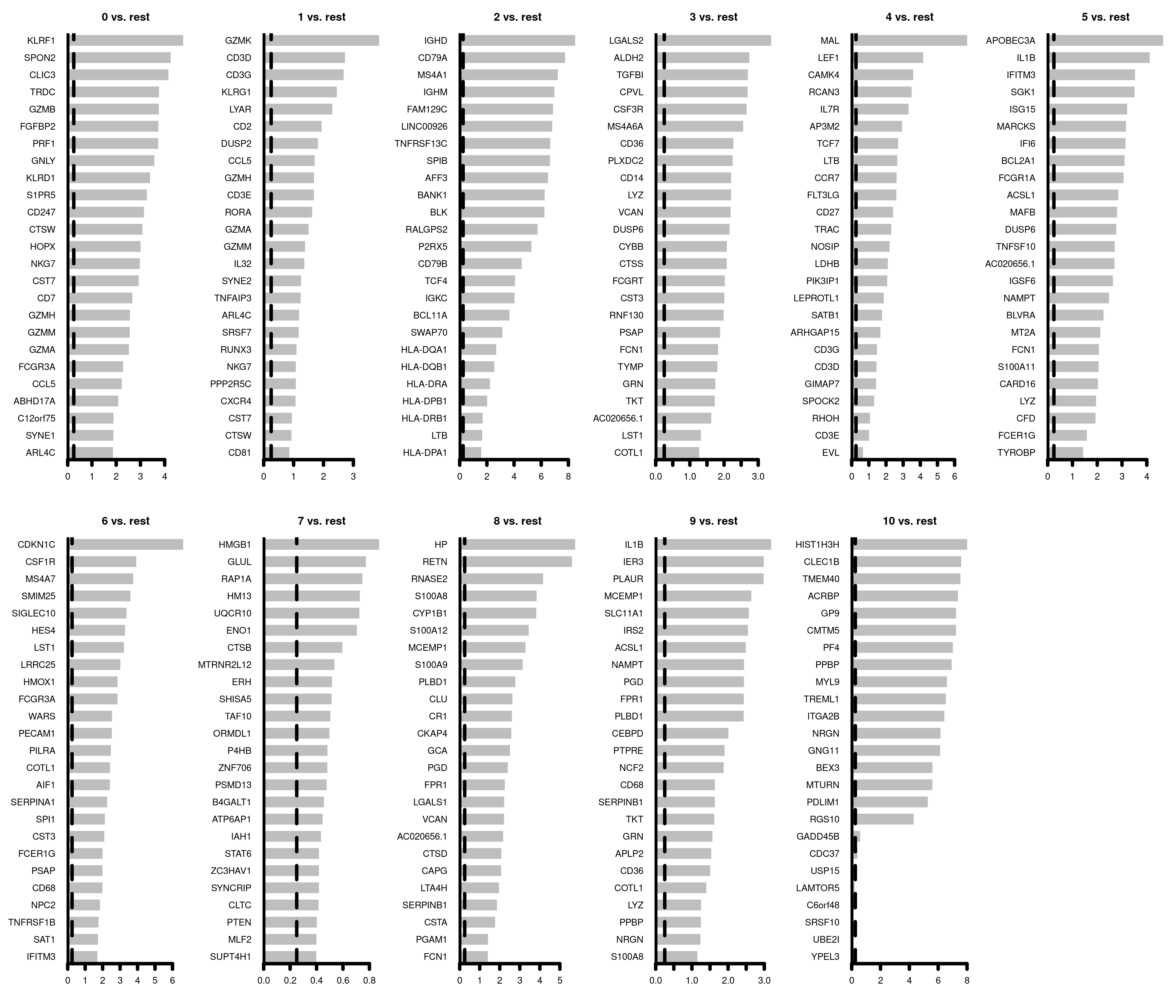
Warning

The plot below is not a ggplot but a basic plot. This is an example how to sometimes utilize a base plot to make elegant plots

par(mfrow = c(2, 6), mar = c(4, 6, 3, 1))
for (i in unique(top25$cluster)) {
    barplot(sort(setNames(top25$avg_log2FC, top25$gene)[top25$cluster == i], F),
        horiz = T, las = 1, main = paste0(i, " vs. rest"), border = "white", yaxs = "i"
    )
    abline(v = c(0, 0.25), lty = c(1, 2))
}

We can visualize them as a heatmap. Here we are selecting the top 5.

markers_genes %>%
    group_by(cluster) %>%
    slice_min(p_val_adj, n = 5, with_ties = FALSE) -> top5
# create a scale.data slot for the selected genes
covid_final <- ScaleData(covid_final, features = as.character(unique(top5$gene)), assay = "RNA")
DoHeatmap(covid_final, features = as.character(unique(top5$gene)), group.by = sel.clust, assay = "RNA")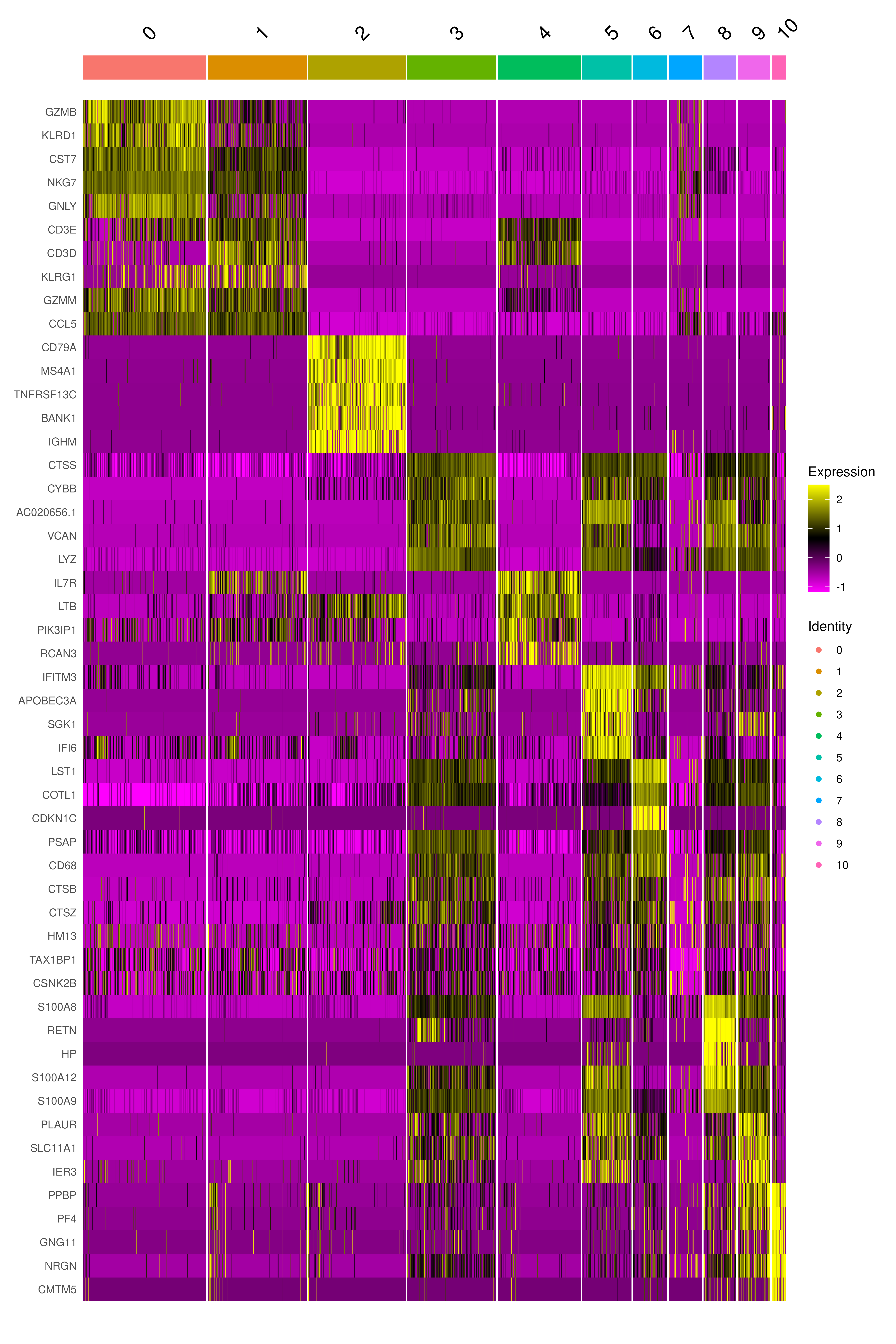

Another way is by representing the overall group expression and detection rates in a dot-plot.

DotPlot(covid_final, features = rev(as.character(unique(top5$gene))), group.by = sel.clust, assay = "RNA") + coord_flip()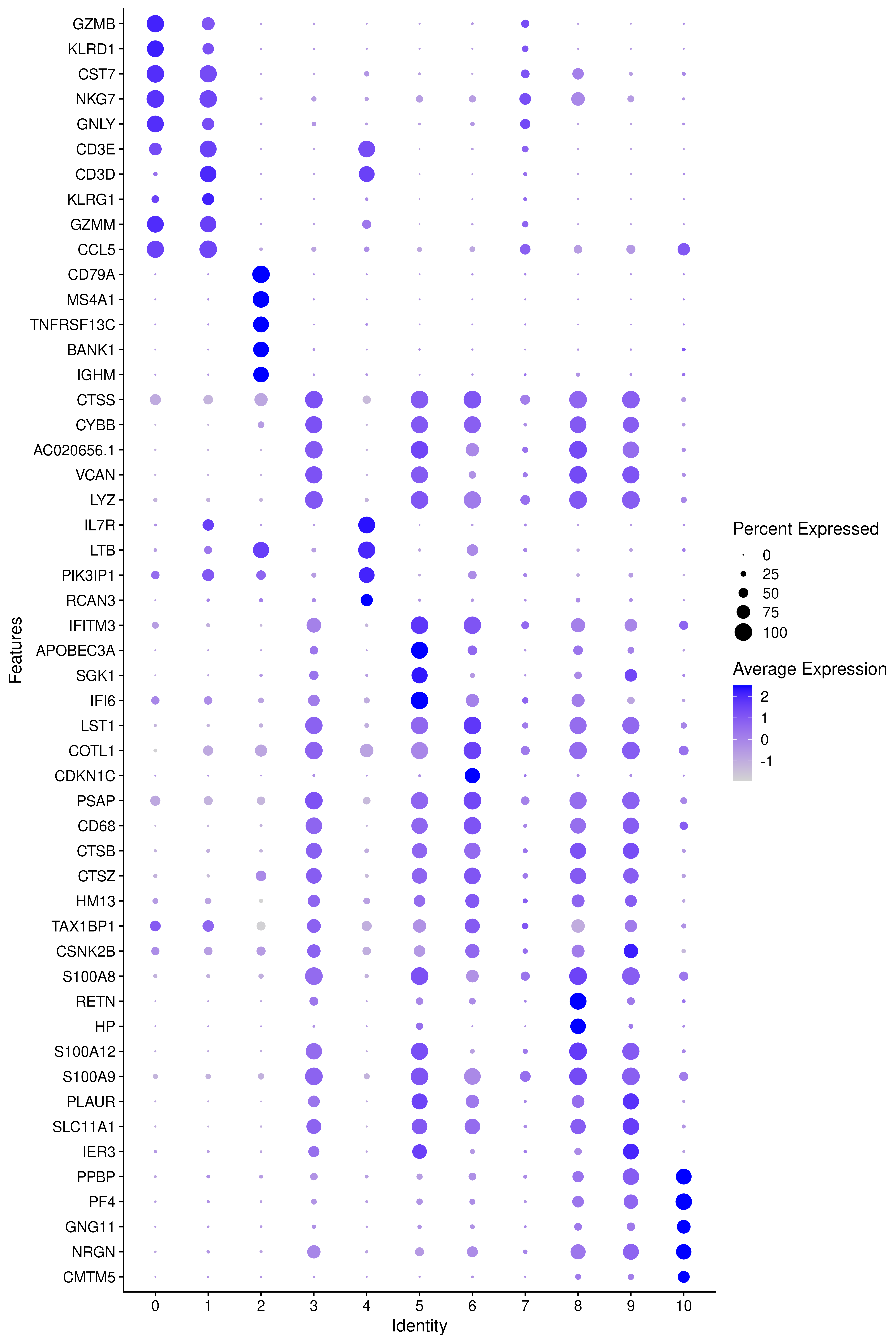

We can also plot a violin plot for each gene.

# take top 3 genes per cluster/
top5 %>%
    group_by(cluster) %>%
    top_n(-3, p_val) -> top3

# set pt.size to zero if you do not want all the points to hide the violin shapes, or to a small value like 0.1
VlnPlot(covid_final, features = as.character(unique(top3$gene)), ncol = 5, group.by = sel.clust, assay = "RNA", pt.size = 0)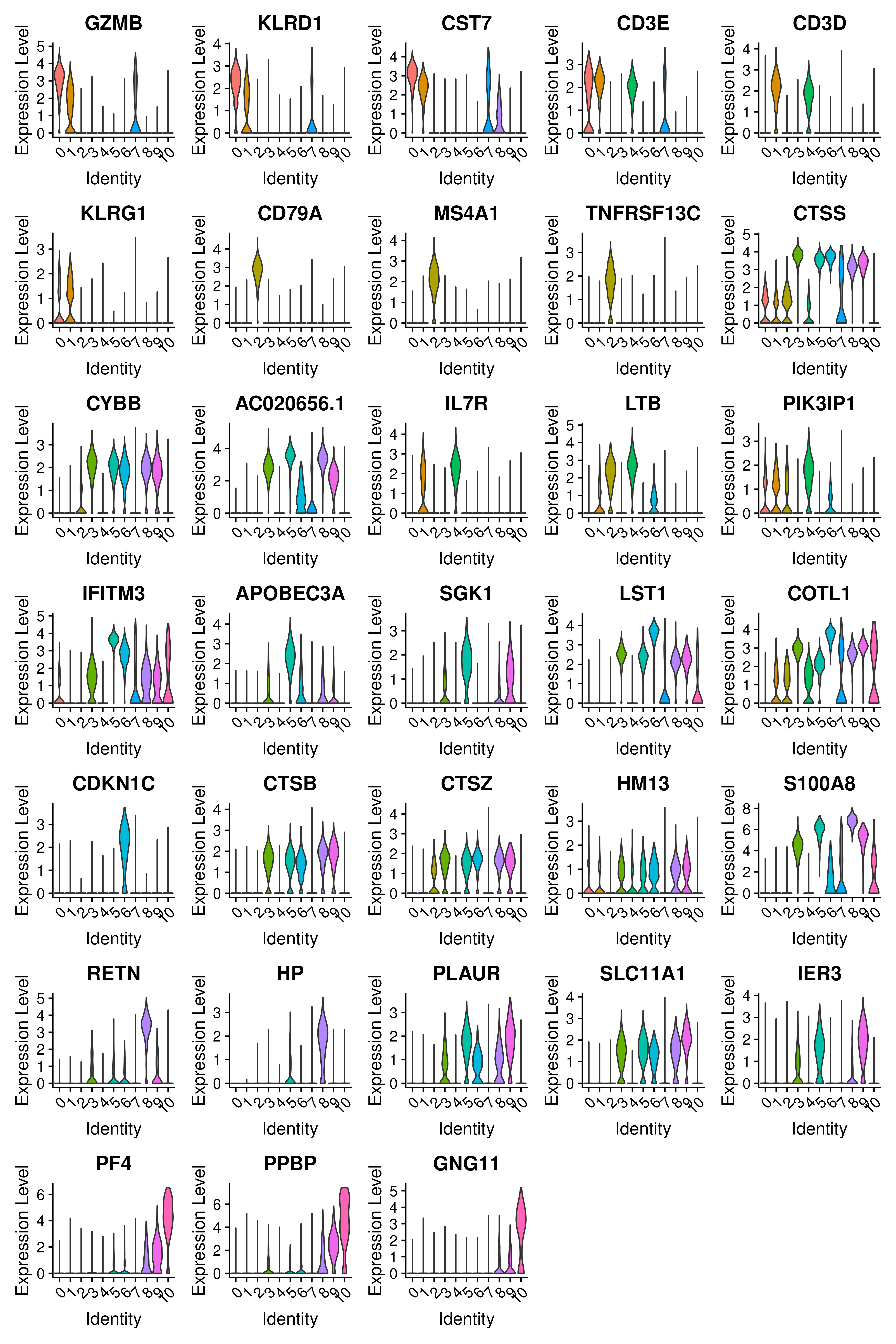

6.2 Covid vs Ctrl

Now, let us assume that you are interested in finding the differentially expressed genes between the patients with Covid vs the Control. We will take here the cluster 2 as it has a good representation of the patients from both conditions. So, we could specifically run the DGE within that cluster like below:

# select all cells in cluster 2
cell_selection <- subset(covid_final, cells = colnames(covid_final)[covid_final@meta.data[, sel.clust] == 2])
cell_selection <- SetIdent(cell_selection, value = "type")
# Compute differentiall expression
DGE_cell_selection <- FindAllMarkers(cell_selection,
    logfc.threshold = 0.2,
    test.use = "wilcox",
    min.pct = 0.1,
    min.diff.pct = 0.2,
    only.pos = TRUE,
    max.cells.per.ident = 50,
    assay = "RNA"
)

We can now plot the expression across the type

DGE_cell_selection %>%
    group_by(cluster) %>%
    top_n(-5, p_val) -> top5_cell_selection
VlnPlot(cell_selection, features = as.character(unique(top5_cell_selection$gene)), ncol = 5, group.by = "type", assay = "RNA", pt.size = .1)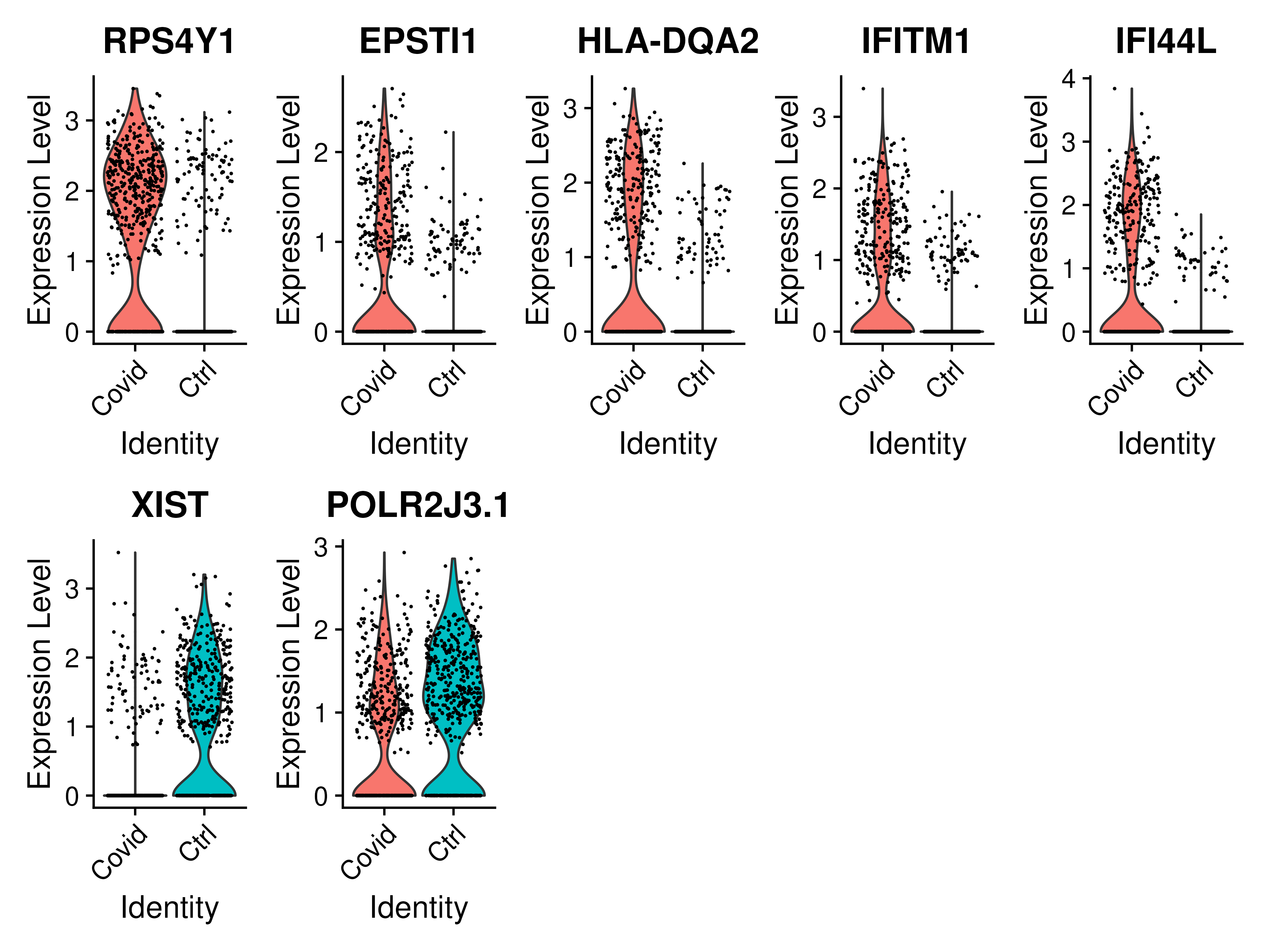

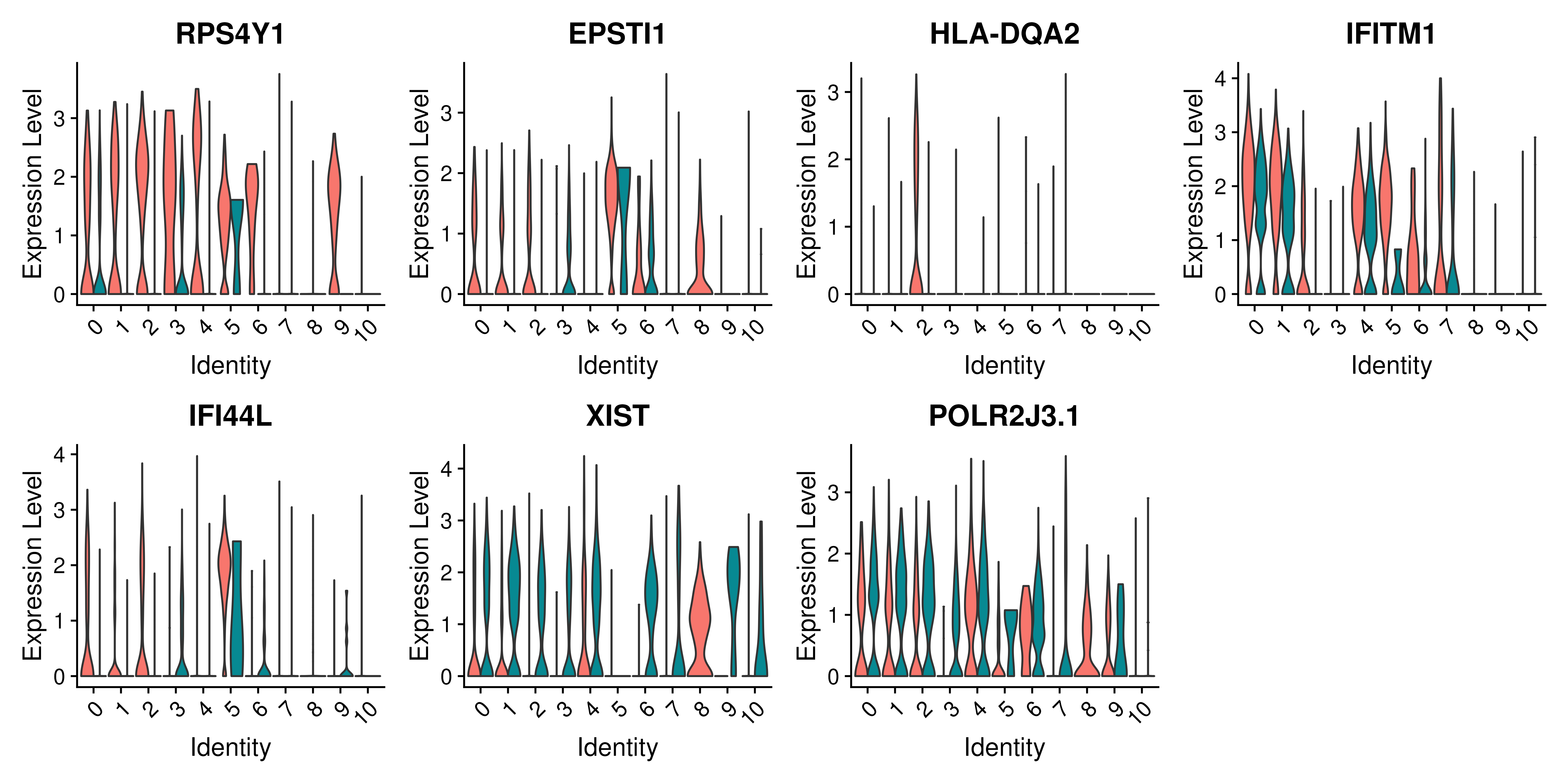
We can also plot these genes across all clusters, but split by type, to check if the genes are also over/under expressed in other celltypes/clusters.

VlnPlot(covid_final,
    features = as.character(unique(top5_cell_selection$gene)),
    ncol = 4, split.by = "type", assay = "RNA", pt.size = 0, split.plot = TRUE
)

7 Acknowledgements

All the material in this section were based on a 5-day workshop given by our NBIS colleagues on the single-cell analysis. We only scratch the surface here to think about the important visualizations one does in relation to single-cell data anaysis. There is much more to the actual analysis and the QC steps in relation to the down stream analysis of any single-cell data. If you have more questions, please go through the material available as part of that workshop