3 Common cases

Let’s go over some common cases of linear models to clarify their interpretation and usage. We will need to run this code to begin with:

library(tidyverse)
library(magrittr)
library(faraway)
library(ggiraphExtra)

font.size <- 12
my.ggtheme <- 
  theme_bw() + 
  theme(axis.title = element_text(size = font.size), 
        axis.text = element_text(size = font.size), 
        legend.text = element_text(size = font.size), 
        legend.title = element_blank(), 
        legend.position = "top")
      

# add obesity and diabetes status to diabetes faraway data
inch2m <- 2.54/100
inch2cm <- 2.54
pound2kg <- 0.45
data_diabetes <- diabetes %>%
  mutate(height  = height * inch2m, height = round(height, 2)) %>% 
  mutate(waist = waist * inch2cm) %>%  
  mutate(weight = weight * pound2kg, weight = round(weight, 2)) %>%
  mutate(BMI = weight / height^2, BMI = round(BMI, 2)) %>% 
  mutate(obese= cut(BMI, breaks = c(0, 29.9, 100), labels = c("No", "Yes"))) %>% 
  mutate(diabetic = ifelse(glyhb > 7, "Yes", "No"), diabetic = factor(diabetic, levels = c("No", "Yes"))) %>%
  na.omit()

3.1 Example: simple linear regression

m1 <- lm(BMI ~ waist, data = data_diabetes)
summary(m1)
## 
## Call:
## lm(formula = BMI ~ waist, data = data_diabetes)
## 
## Residuals:
##      Min       1Q   Median       3Q      Max 
## -13.2374  -2.7689  -0.4532   2.4065  19.3549 
## 
## Coefficients:
##             Estimate Std. Error t value Pr(>|t|)    
## (Intercept) -5.12445    2.73538  -1.873   0.0633 .  
## waist        0.35298    0.02723  12.965   <2e-16 ***
## ---
## Signif. codes:  0 '***' 0.001 '**' 0.01 '*' 0.05 '.' 0.1 ' ' 1
## 
## Residual standard error: 4.426 on 128 degrees of freedom
## Multiple R-squared:  0.5677, Adjusted R-squared:  0.5643 
## F-statistic: 168.1 on 1 and 128 DF,  p-value: < 2.2e-16

ggPredict(m1) + 
  my.ggtheme + 
  xlab("waist [cm]")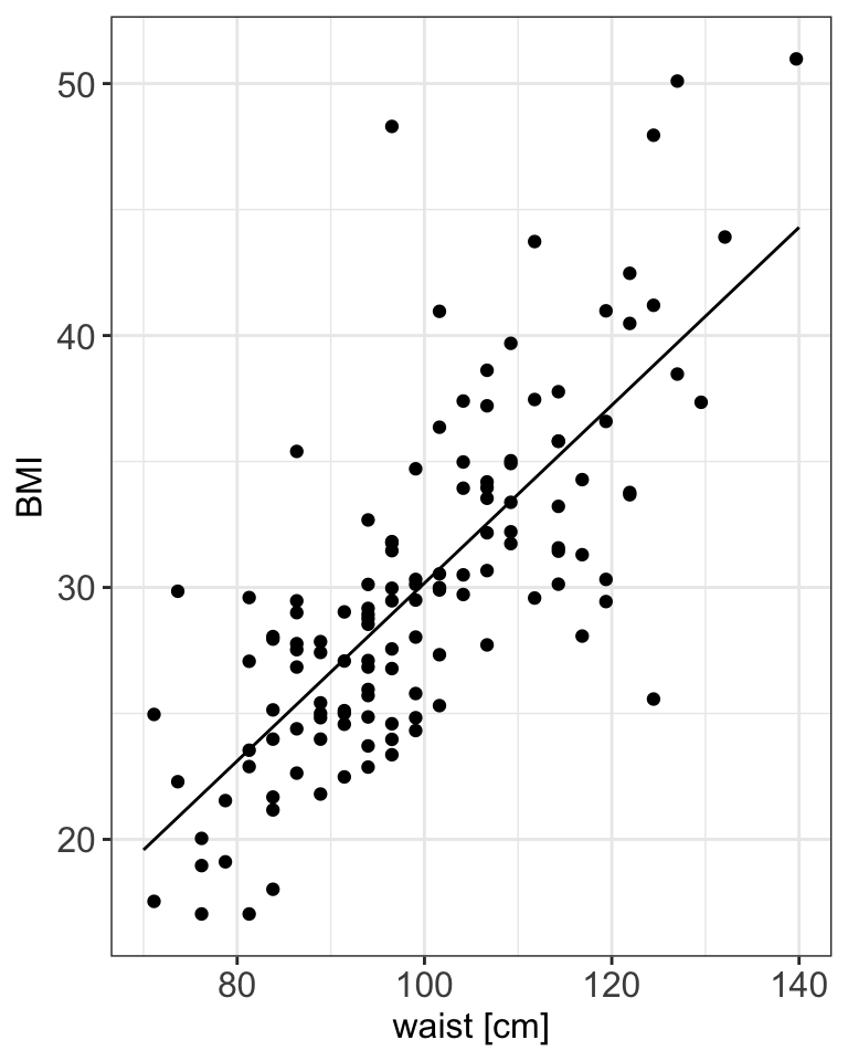

Figure 3.1: Scatter plot showing BMI values given waist measurments with a fitted simple linear regression model.

Model (generic)

$Y_i = \alpha + \beta \cdot x_i + \epsilon_i$

Model (fitted)

$BMI_i = -5.12 + 0.35 \cdot waist_i + \epsilon_i$

Slope

The value of slope tells us how and by much the outcome changes with a unit change in $x$
If the waist increases by 1 unit, here in cm, what would be our expected change in BMI¹$?
And if the waist increases by 10 units what would be our expected change in BMI²$?

Intercept

The intercept, often labeled the constant, is the value of Y when $x_i=0$.
In models where $x_i$ can be equal 0, the intercept is simply the expected mean value of response.
In models where $x_i$ cannot be equal 0, like in our BMI example where it is not possible to have BMI equal to zero, the intercept has no intrinsic meaning.
The intercept is thus quite often ignored in linear models, as it is the value of slope that dictates the association between exposure and outcome.

Hypothesis testing

We’ve seen during the lecture that the check for association between exposure and outcome we check if the we have enough evidence to reject $H_0: \beta=0$ in favor of the alternative $H_a: \beta\neq0$.
Here, for the $\beta$ coefficient we have $t-statistics = 0.35298 / 0.02723 = 12.965$ and a corresponding $p-value = 12.96291$, as $t-statistics \sim t(130-2) << 0.05$. Such large t-statsitics or small p-value means we have enough evidence to reject the null hypothesis and conclude that there is a significant association between waist and BMI.
We can double-check R output by calculating p-value ourselves using the Student t distribution:

2*pt(12.96291, df=128, lower=F)
## [1] 4.605102e-25

Is there enough evidence to reject the null hypothesis of $H_0: \alpha=0$ in favor of the alternative $H_a: \alpha\neq0$ assuming 5% significance level?³.
Is there enough evidence to reject the null hypothesis of $H_0: \alpha=0$ in favor of the alternative $H_a: \alpha\neq0$ assuming 10% significance level?⁴.

Predictions

Using the model we can predict the BMI value for a new observation of waist.
For instance, we can find expected BMI value for someone who measures 100 cm in waist by:
$BMI = -5.12445 + 0.35298 \cdot 100 = 30.17355$
In R can use predict() function:

# predict BMI for a new value of 100
new_data <- data.frame(waist = 100)
predict(m1, newdata = new_data)
##        1 
## 30.17348

What would be BMI for someone with waist measurements of 75?⁵
What would be BMI for someone with waist measurements of 200?⁶

Model fit

In simple regression we can use $R^2$ to assess model fit, here $R^2 = 0.5677$.
Do you think that the model fits the data well?⁷

Model assumptions

We should also not forget to look at the residual plots to check model assumptions:

Code

par(mfrow = c(2,2))
plot(m1)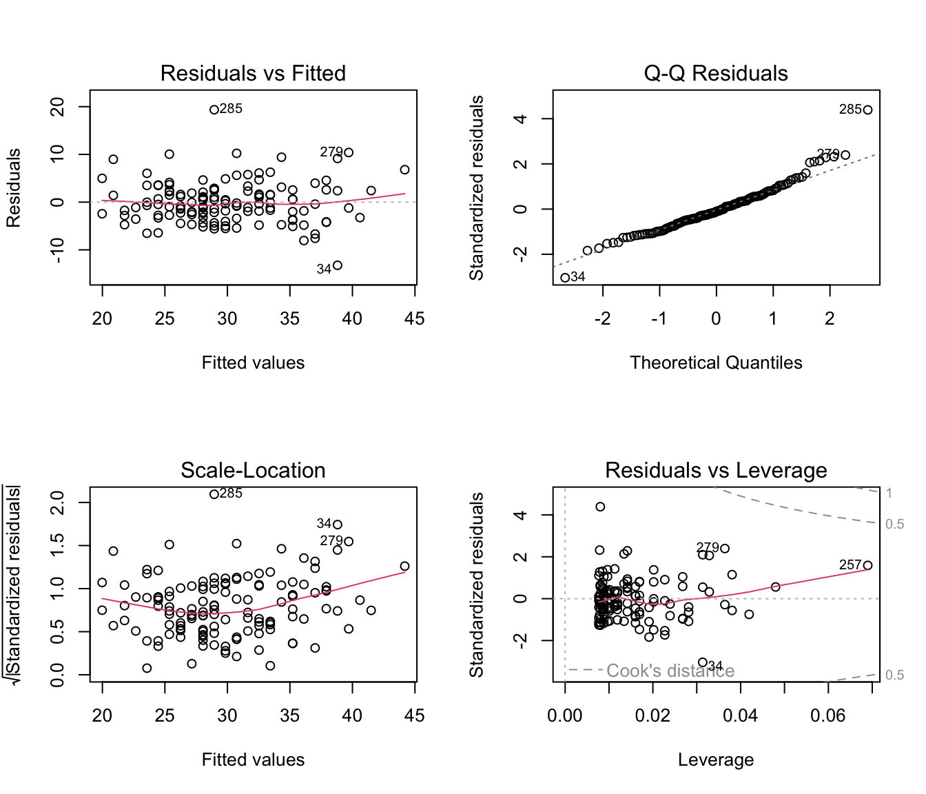

Given the diagnostic plots can we comment about the assumptions of linear models being met?⁸

3.2 Example: multiple regression

Let’s try to model BMI using more variables

Model (generic)

$Y_i = \beta_0 + \beta_1 \cdot age_i + \beta_2 \cdot chol_i + \beta_3 \cdot hdl_i + \epsilon_i$

# fit multiple linear regression and print model summary
m2 <- lm(BMI ~ age + chol + hdl,  data = data_diabetes)
summary(m2)
## 
## Call:
## lm(formula = BMI ~ age + chol + hdl, data = data_diabetes)
## 
## Residuals:
##     Min      1Q  Median      3Q     Max 
## -13.074  -4.833  -1.132   3.438  22.032 
## 
## Coefficients:
##              Estimate Std. Error t value Pr(>|t|)    
## (Intercept) 35.456968   3.149661  11.257  < 2e-16 ***
## age         -0.027047   0.040304  -0.671  0.50340    
## chol         0.002039   0.012701   0.161  0.87269    
## hdl         -0.090023   0.032734  -2.750  0.00683 ** 
## ---
## Signif. codes:  0 '***' 0.001 '**' 0.01 '*' 0.05 '.' 0.1 ' ' 1
## 
## Residual standard error: 6.552 on 126 degrees of freedom
## Multiple R-squared:  0.06763,    Adjusted R-squared:  0.04543 
## F-statistic: 3.046 on 3 and 126 DF,  p-value: 0.03124

Coefficient interpretations

Using the model answer the questions:

what would happen to BMI if hdl levels increase by 10?⁹
what would happen to BMI if age increases by 1 year?¹⁰

Hypothesis testing

overall, is there a relationship between the response $Y$ (BMI) and predictors?¹¹

Not so easy: alternative model

Let’s consider another multiple regression model:

$Y_i = \beta_0 + \beta_1 \cdot age_i + \beta_2 \cdot chol_i + \beta_3 \cdot hdl_i + \beta_4 \cdot waist_i + \epsilon_i$

We fit the model in R and look at the model summary:

m2_alt <- lm(BMI ~ age + chol + hdl + waist, data = data_diabetes)
summary(m2_alt)
## 
## Call:
## lm(formula = BMI ~ age + chol + hdl + waist, data = data_diabetes)
## 
## Residuals:
##      Min       1Q   Median       3Q      Max 
## -13.0337  -3.0416  -0.6777   2.2711  18.2894 
## 
## Coefficients:
##              Estimate Std. Error t value Pr(>|t|)    
## (Intercept) -0.921431   3.588473  -0.257   0.7978    
## age         -0.050397   0.027016  -1.865   0.0645 .  
## chol        -0.006250   0.008519  -0.734   0.4645    
## hdl         -0.006199   0.022890  -0.271   0.7870    
## waist        0.353256   0.028213  12.521   <2e-16 ***
## ---
## Signif. codes:  0 '***' 0.001 '**' 0.01 '*' 0.05 '.' 0.1 ' ' 1
## 
## Residual standard error: 4.381 on 125 degrees of freedom
## Multiple R-squared:  0.5864, Adjusted R-squared:  0.5732 
## F-statistic:  44.3 on 4 and 125 DF,  p-value: < 2.2e-16

What happens to BMI if hdl increases by 10?¹²
What happens to BMI if hdl increases by 10 using the first model again?[decreases by ca. 0.9]
How do you explain the difference in BMI changes given these two models?

Specific interpretation

Obviously there is difference between decrease of 0.9 BMI and decrease of 0.06 in BMI (alternative model).
Our interpretations need to be more specific and we say that a unit increase in $x$ with other predictors held constant will produce a change equal to $\hat{\beta}$ in the response $y$
Often it may be quite unrealistic to be able to control other variables and keep them constant and for our alternative model, a change in hdl would also imply a change in total cholesterol chol.
Further, our explanation contains no notation of causation.
We will learn later how to choose the best model by assessing its fit and including only relevant variable (feature selection), for now we focus on learning how to interpret the coefficients given a fitted model.

3.3 Example: categorical variable

We want to compare the average BMI of men and women.
We can do that using linear regression and including gender as binary variable

Code

font.size <- 20
col.blue.light <- "#a6cee3"
col.blue.dark <- "#1f78b4"
my.ggtheme <- 
  theme_bw() + 
  theme(axis.title = element_text(size = font.size), 
        axis.text = element_text(size = font.size), 
        legend.text = element_text(size = font.size), 
        legend.title = element_blank(), 
        legend.position = "top")
      

# visualize the data with box plot
data_diabetes %>%
  ggplot(aes(x = gender, y = BMI, fill = gender)) + 
  geom_boxplot() + 
  scale_fill_brewer(palette = "Set2") + 
  my.ggtheme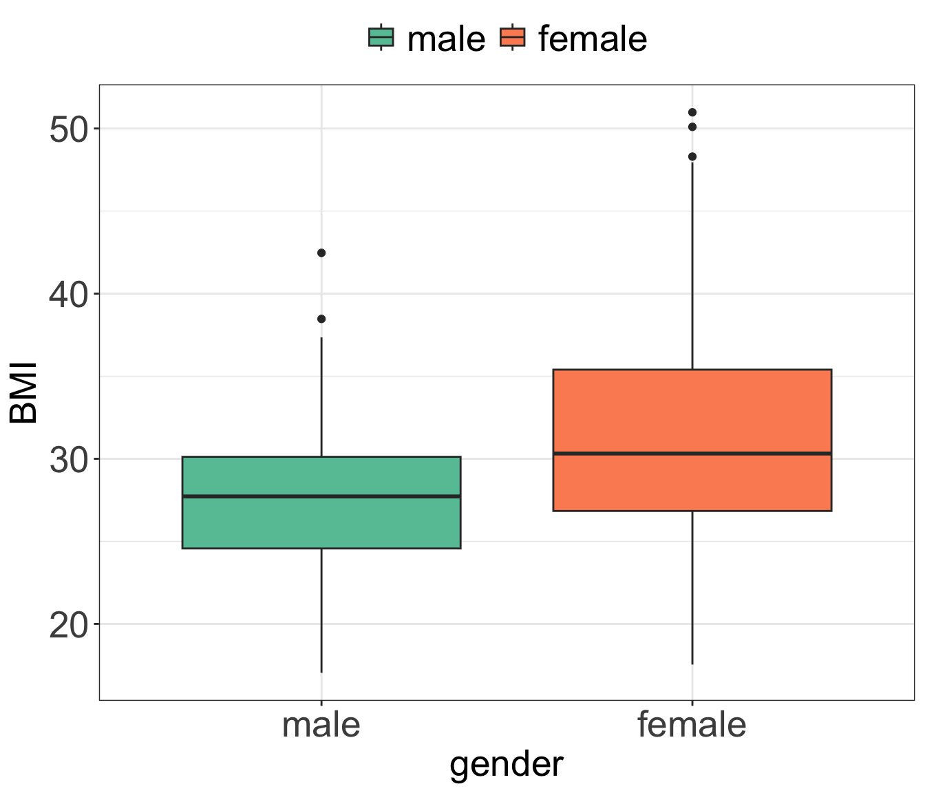

Model

\[Y_i = \alpha + \beta I_{x_i} + \epsilon_i\] where \[\begin{equation} I_{x_i} = \left\{ \begin{array}{cc} 1 & \mathrm{if\ } x_i=1 \\ 0 & \mathrm{if\ } x_i=0 \\ \end{array} \right. \end{equation}\] for some coding, e.g. we choose to set “Female=1” and “Male=0” or vice versa.

In R we write:

# Note: check that Gender is indeed non-numeric
print(class(data_diabetes$gender))
## [1] "factor"

# fit linear regression and print model summary
m3 <- lm(BMI ~ gender, data = data_diabetes)
print(summary(m3))
## 
## Call:
## lm(formula = BMI ~ gender, data = data_diabetes)
## 
## Residuals:
##     Min      1Q  Median      3Q     Max 
## -14.167  -4.117  -0.327   3.160  19.273 
## 
## Coefficients:
##              Estimate Std. Error t value Pr(>|t|)    
## (Intercept)   27.7674     0.8527  32.566  < 2e-16 ***
## genderfemale   3.9396     1.1379   3.462 0.000729 ***
## ---
## Signif. codes:  0 '***' 0.001 '**' 0.01 '*' 0.05 '.' 0.1 ' ' 1
## 
## Residual standard error: 6.437 on 128 degrees of freedom
## Multiple R-squared:  0.08563,    Adjusted R-squared:  0.07849 
## F-statistic: 11.99 on 1 and 128 DF,  p-value: 0.0007286

Estimates \[\hat{\alpha} = 27.7674\] \[\hat{\beta} = 3.9396\]

The lm() function chooses automatically one of the category as baseline, here females.
Model summary prints the output of the model with the baseline category “hidden”.
Notice that the only label we have is “genderfemale”.
Meaning that we ended-up having a model coded as below: \[\begin{equation} I_{x_i} = \left\{ \begin{array}{cc} 1 & \mathrm{if\ } \quad person_i\;is\;female \\ 0 & \mathrm{if\ } \quad person_i\;is\;male \\ \end{array} \right. \end{equation}\]
Consequently, if observation $i$ is female then the expected value of BMI is: \[E(BMI_i|female) = 27.7674 + 3.9396 = 31.707\]
and if observation $i$ is male then the expected value of BMI is: \[E(BMI_i|male) = 27.7674\] We can plot the model in R:

ggPredict(m3) + 
  my.ggtheme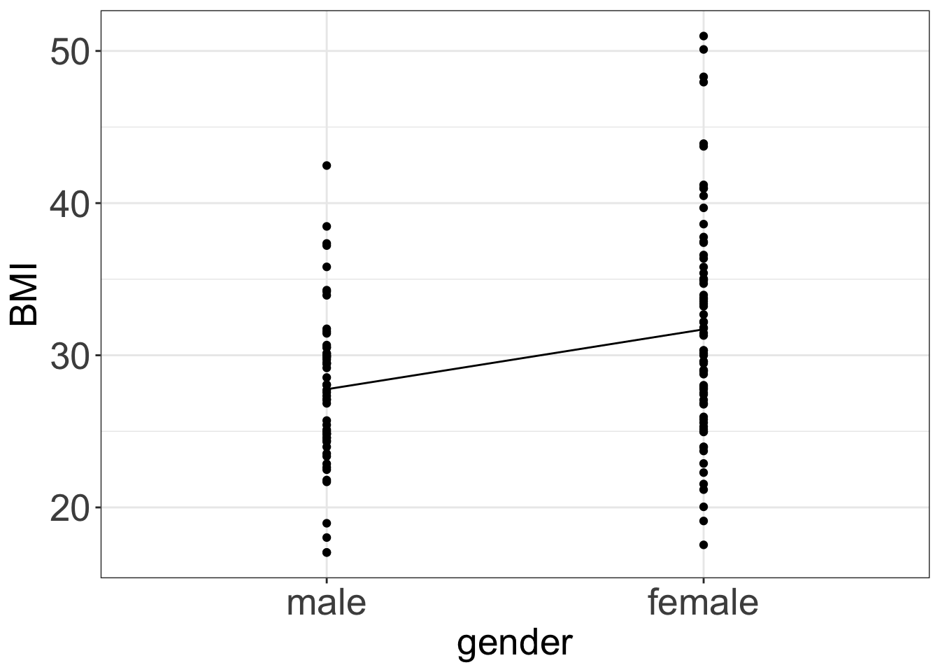

3.4 Example: categorical & numerical variables

Above we observed a signficant difference in average BMI between men and women among the study participants.
Can we also observe a significant relationship between BMI and height?
And if so, does this relationship depend on gender?

Code

#|label: fig-htwtgen-plot
#|fig-cap: Scatter plot showing BMI measurments given height stratified by gender.
#|fig-cap-location: margin
#|collapse: true
#|code-fold: false
#|fig-width: 5
#|fig-heigth: 5

# plot the data separately for Male and Female
data_diabetes %>%
  ggplot(aes(x = height, y=BMI, col = gender)) +
  geom_point(alpha = 0.8, size = 3) +
  scale_color_brewer(palette = "Set2") + 
  my.ggtheme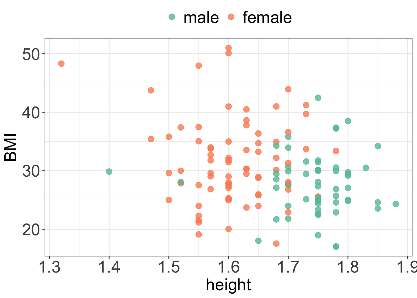

From the plot we can see that BMI decreases slightly with height.
On average, men are taller than women.
On average, women have higher BMI than men.
The relationship between height and BMI appears to be the same for males and females, i.e. BMI decreases with height for both men and women.

To assess the relationship we use a model containing height and gender.

Model

\[Y_i = \alpha + \beta I_{x_i} + \gamma x_{2,i} + \epsilon_i\] where \[\begin{equation} I_{x_i} = \left\{ \begin{array}{cc} 1 & \mathrm{if\ } \quad person_i\;is\;female \\ 0 & \mathrm{if\ } \quad person_i\;is\;male \\ \end{array} \right. \end{equation}\]

and $x_{2,i}$ is the height of person $i$.

In R we write:

# fit linear model and print model summary
m4 <- lm(BMI ~ gender + height, data = data_diabetes)
print(summary(m4))
## 
## Call:
## lm(formula = BMI ~ gender + height, data = data_diabetes)
## 
## Residuals:
##      Min       1Q   Median       3Q      Max 
## -13.7580  -4.2617  -0.3863   3.1646  19.2244 
## 
## Coefficients:
##              Estimate Std. Error t value Pr(>|t|)   
## (Intercept)    37.743     13.294   2.839  0.00527 **
## genderfemale    3.163      1.538   2.057  0.04172 * 
## height         -5.719      7.606  -0.752  0.45350   
## ---
## Signif. codes:  0 '***' 0.001 '**' 0.01 '*' 0.05 '.' 0.1 ' ' 1
## 
## Residual standard error: 6.448 on 127 degrees of freedom
## Multiple R-squared:  0.08969,    Adjusted R-squared:  0.07535 
## F-statistic: 6.256 on 2 and 127 DF,  p-value: 0.002562

Model together with estimates

\[Y_i = \alpha + \beta I_{x_i} + \gamma x_{2,i} + \epsilon_i\] where \[\begin{equation} I_{x_i} = \left\{ \begin{array}{cc} 1 & \mathrm{if\ } \quad person_i\;is\;male \\ 0 & \mathrm{if\ } \quad person_i\;is\;female \\ \end{array} \right. \end{equation}\]

and $x_{2,i}$ is the weight of person $i$

Estimates

\[\hat{\alpha} = 37.743 \] \[\hat{\beta} = 3.163\] \[\hat{\gamma} = -5.719\]

For instance, using our estimates, for a female who happens to 1.7 m tall we would predict BMI of: \[E(BMI_i|female, height = 1.7) = 37.743 + 3.163 + (-5.719 \cdot 1.7) = 31.1837\]
and for a male of height 1.7 m tall we would predict BMI of \[E(BMI_i|male, height = 1.7) = 37.743 + (-5.719 \cdot 1.7) = 28.0207\]

In R we can plot our data and the fitted model to verify our calculations:

# plot the data separately for men and women
# using ggplot() and geom_smooth()
ggPredict(m4) + 
  scale_color_brewer(palette = "Set2") + 
  my.ggtheme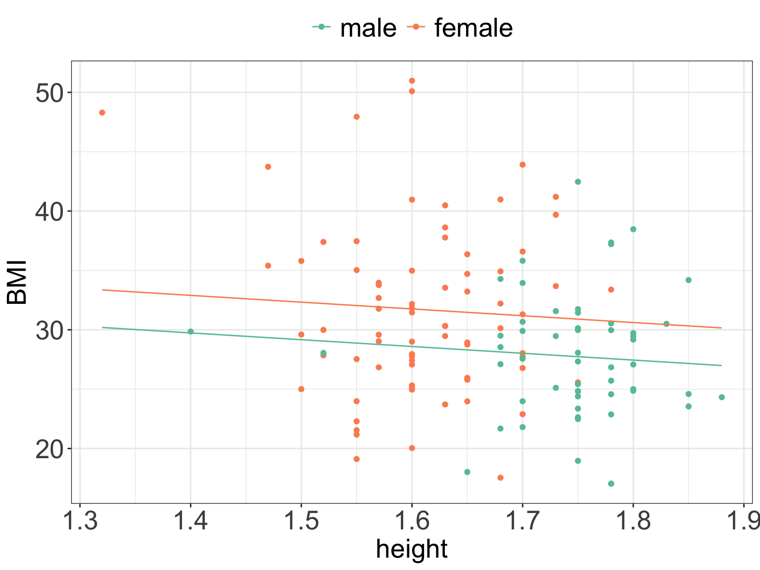

3.5 Example: interactions

The fitted lines in the above example are parallel, the slope is modeled to be the same for men and women, and the intercept denotes the group differences.
It is also possible to allow for both intercept and slope being fitted separately for each group.
This is done when we except that the relationships are different in different groups, e.g. increasing in one group and decreasing in the other.
And we then talk about including interaction effect since the two lines may interact (cross).

Model

\[Y_{i,j} = \alpha_i + \beta_ix_{ij} + \epsilon_{i,j}\] where:

$Y_{i,j}$ is the BMI of person $j$ of gender $i$
$x_{ij}$ is the height of person $j$ of gender $i$
$i=1$ corresponds to women in our example (keeping the same coding as above)
$i=2$ corresponds to men

In R we define the interaction term with *:

# fit linear model with interaction
m5 <- lm(BMI ~ gender * height, data = data_diabetes)
print(summary(m5))
## 
## Call:
## lm(formula = BMI ~ gender * height, data = data_diabetes)
## 
## Residuals:
##      Min       1Q   Median       3Q      Max 
## -13.5564  -4.1137  -0.3072   3.1057  19.2005 
## 
## Coefficients:
##                     Estimate Std. Error t value Pr(>|t|)
## (Intercept)           31.222     20.318   1.537    0.127
## genderfemale          14.219     26.032   0.546    0.586
## height                -1.981     11.638  -0.170    0.865
## genderfemale:height   -6.558     15.414  -0.425    0.671
## 
## Residual standard error: 6.469 on 126 degrees of freedom
## Multiple R-squared:  0.09099,    Adjusted R-squared:  0.06935 
## F-statistic: 4.204 on 3 and 126 DF,  p-value: 0.007155

Now, based on the regression output we would expect:

for a woman of height $x$, a BMI value of: \[E(BMI|female\; and \; height=x)=31.222 + 14.219 - 1.981 \cdot x - 6.558 \cdot x = 45.441 -8.539 \cdot x\]
for a man of height $x$, a BMI value of \[E(BMI|male\; and \; height=x)=31.222-1.981 \cdot x\]

Estimates \[\hat{\alpha_1} = 45.441\] \[\hat{\beta_1} = 31.222\]

\[\hat{\alpha_2} = 47.34778\] \[\hat{\beta_2} = -1.981\]

We can see from the regression output that there is no evidence to reject the null hypothesis that the interaction term “Genderfemale:height” is equal to zero.
Or therefore conclude that the relationship between BMI and height is different for men and women.
We can plot the fitted model and see that the lines are no longer parallel.

ggPredict(m5) +
  guides(color=guide_legend(override.aes=list(fill=NA))) + 
  scale_color_brewer(palette = "Set2") + 
  my.ggtheme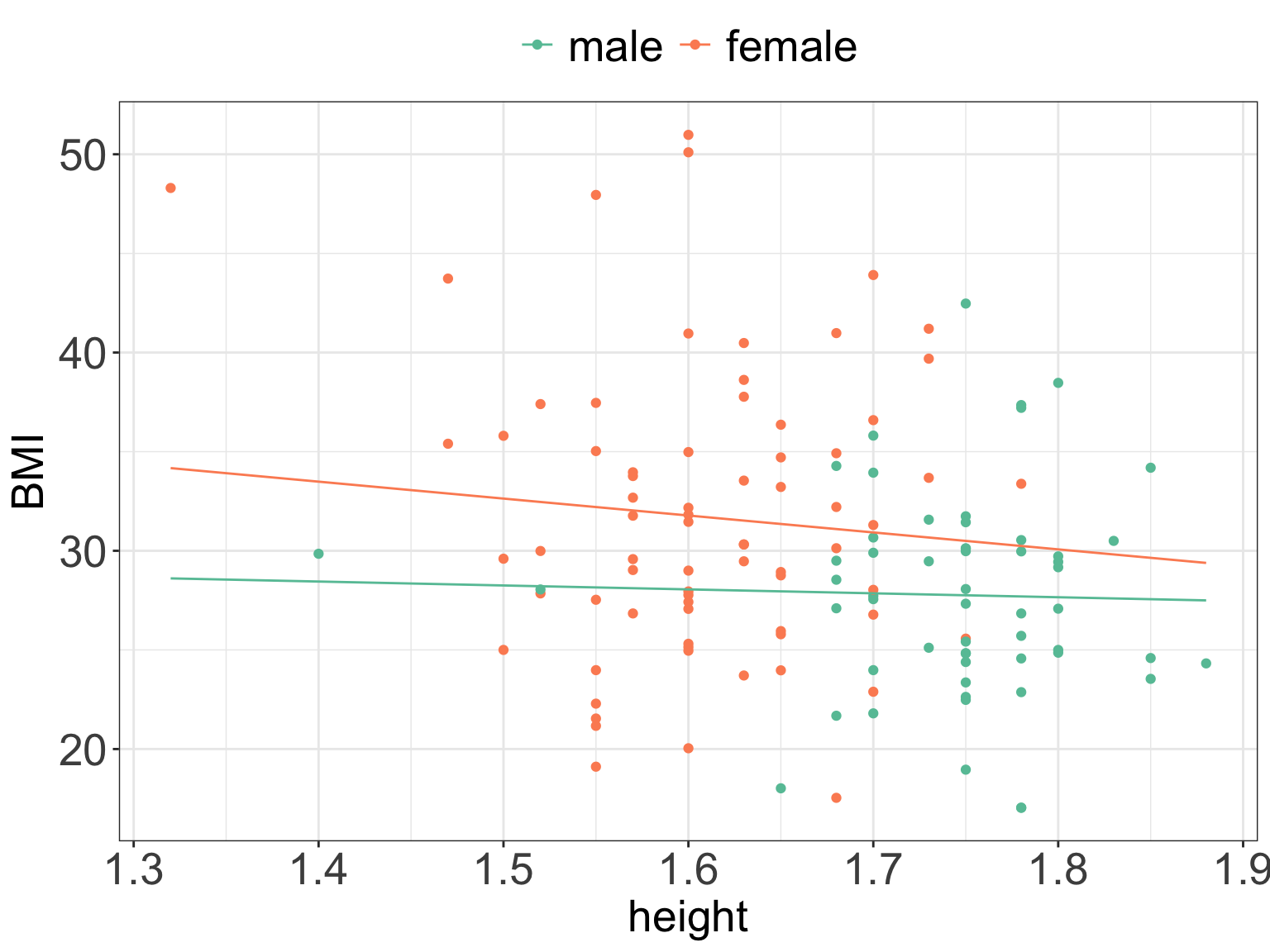

3.6 Example: logistic regression with categorical variable

# recode diabetic status to 1 and 0
data_diabetes <- data_diabetes %>%
  mutate(obese = ifelse(obese == "Yes", 1, 0))

# fit logistic regression using age and gender
m6 <- glm(obese ~  hdl + gender, family = binomial(link="logit"), data = data_diabetes)
summary(m6)
## 
## Call:
## glm(formula = obese ~ hdl + gender, family = binomial(link = "logit"), 
##     data = data_diabetes)
## 
## Coefficients:
##              Estimate Std. Error z value Pr(>|z|)   
## (Intercept)   0.55047    0.58718   0.937   0.3485   
## hdl          -0.02997    0.01197  -2.504   0.0123 * 
## genderfemale  1.26586    0.40120   3.155   0.0016 **
## ---
## Signif. codes:  0 '***' 0.001 '**' 0.01 '*' 0.05 '.' 0.1 ' ' 1
## 
## (Dispersion parameter for binomial family taken to be 1)
## 
##     Null deviance: 178.71  on 129  degrees of freedom
## Residual deviance: 164.39  on 127  degrees of freedom
## AIC: 170.39
## 
## Number of Fisher Scoring iterations: 4

By how much change odds of suffering from obesity when hdl increases by 1?¹³
What are the odds of suffering from obesity and being a women vs. suffering from obesity and being a man?¹⁴

ggPredict(m6) + 
  scale_color_brewer(palette = "Set2") + 
  my.ggtheme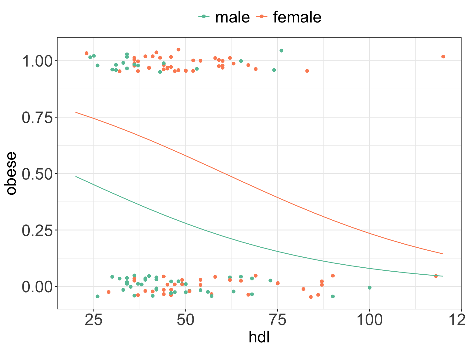

We can predict obesity status in R for a man with hdl values of 50:

# define new observation
df <- data.frame(hdl = 50, gender = as.factor("male"))

# predict probability of suffering from obesity
prob_obese <- predict(m6, newdata = df, type = "response")
print(prob_obese)
##         1 
## 0.2792396

If the waist increases by 1 cm we would expect our BMI to increase by $\approx 0.35$ since $\hat{\beta} = 0.35298$↩︎
If the waist increases by 10 cm we would expect BMI to increase by $0.35298 \cdot 10 \approx 3.53$↩︎
No, as $p-value = 0.0633 \nless 0.05$↩︎
Yes, as $p-value = 0.0633 < 0.1$↩︎
BMI = -5.12445 + 0.35298 = 21.349↩︎
BMI = -5.12445 + 0.35298 = 65.47141, however here we have to be careful in predicting outside the model range.↩︎
In simple linear regression $R^2$ is the same as $r^2$ and a value of 0.5677 indicates moderate fit, that agrees with the plot above. Since we have more variables in the data set we could try to improve the fit by including more variables.↩︎
The diagnostics do not indicate a serious violation of model assumptions, with no obvious trends of any kind in the residuals plots. Few samples deviate from diagonal line on the Normal Q-Q plot and these could be removed to ensure that the residuals follow normal distribution.↩︎
decreases by $-0.090023 \cdot 10 = 0.90023$↩︎
decrease by 0.027047, however here we can see that the age coefficient is not significant and therefore we should be careful with our interpretations as there is no evidence that this coefficient is different than 0.↩︎
we have seen before that in the case of simple linear regression it was enough to test the null hypothesis of $H_0: \beta=0$ versus $H_0: \beta\neq0$ to answers the question whether there is an overall relationship between response and predictor. In case of multiple regression, with many predictors, we need to test the null hypothesis of \[H_0: \beta_1 = \beta_2 = \dots = \beta_p = 0\] versus the alternative \[H_a: at \; least \; one \; \beta_j \; is \; non-zero\] This hypothesis test is performed by computing F-statistics reported in the model summary and calculated as $F = \frac{(TSS - RSS)/p}{RSS/(n-p-1)}$ where $TSS = \sum(y_i - \bar{y})^2$ and $RSS = \sum(y_i - \hat{y_i})^2$. Here, the $F-statsitics = 3.046$ and the associated $p-value < 0.05$ so there is enough evidence to reject the null hypothesis in favor of the alternative and conclude that there is an overall significant relationship between response (BMI) and predictors.↩︎
decreases by ca. 0.06↩︎
the odds increase by e^{-0.02997} = 0.97↩︎
The odds of suffering from obesity as a woman are e^{1.26586} = 3.55 times of that suffering from obesity and being a man.↩︎