Data Quality Assessment

Exercises

Task 1.

What is a k-mer?

Solution - click to expand

A sequence of characters of length k.

Task 2.

How many 4-mers are in the following sequence?

ACGTTTATCCTATACGGTAATAC

Solution - click to expand

20 (L-k+1)=(23-4+1)

Task 3.

What are the frequencies of the 4-mers in the sequence above.

Solution - click to expand

ACGT 1	CGTT 1	GTTT 1	TTTA 1	TTAT 1
TATC 1	ATCC 1	TCCT 1	CCTA 1	CTAT 1
TATA 1	ATAC 2	TACG 1	ACGG 1	CGGT 1
GGTA 1	GTAA 1	TAAT 1	AATA 1

Task 4.

Load Kat with the following command:

source /proj/sllstore2017027/workshop-GA2018/tools/anaconda/miniconda2/etc/profile.d/conda.sh
conda activate GA2018
kat --help

Use kat hist to obtain a histogram of data Enterococcus_faecalis/SRR492065_{1,2}.fastq.gz. What is the approximate k-mer coverage? Is anything wrong with this histogram?

# Make a named pipe and run in the background
TMPFILE=$(mktemp -u --suffix ".fastq")
mkfifo "$TMPFILE" && zcat "$READ1" "$READ2" > "$TMPFILE" &
# Run KAT reading from the named pipe
kat hist -t "$CPUS" -o "${PREFIX}.hist" "$TMPFILE"
rm "$TMPFILE"

Solution - click to expand

CPUS=${SLURM_NPROCS:-10}
READ1=Enterococcus_faecalis/SRR492065_1.fastq.gz
READ2=Enterococcus_faecalis/SRR492065_2.fastq.gz
PREFIX=$(basename ${READ1%_1.*} )
TMPFILE=$(mktemp -u --suffix ".fastq")
mkfifo "$TMPFILE" && zcat "$READ1" "$READ2" > "$TMPFILE" &
kat hist -t "$CPUS" -o "${PREFIX}.hist" "$TMPFILE"
rm "$TMPFILE"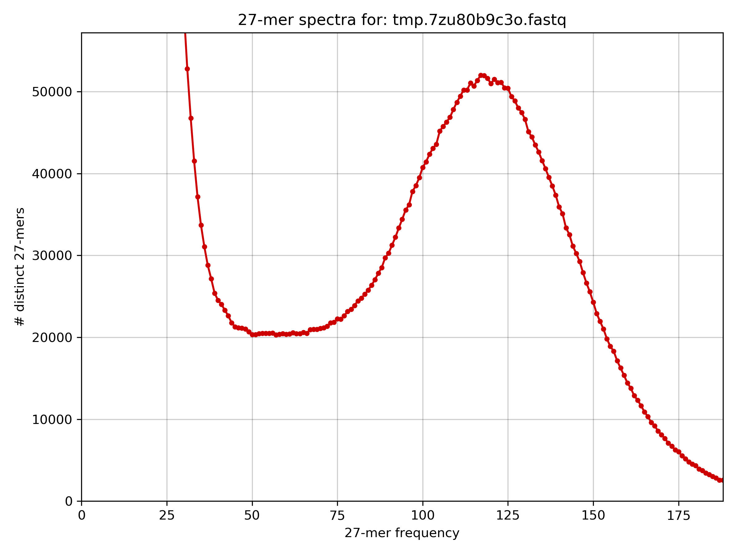

A k-mer histogram of the SRR492065 data.

The homozygous peak in the histogram is at 116x k-mer coverage.

The histogram is unusual because there is a higher than expected frequency of low frequency k-mers.

Task 5.

Use the histogram to estimate the genome size from the homozygous peak. Does this correspond to the estimated genome size of Enterococcus faecalis?

Solution - click to expand

The peak of the histogram is at around 116x coverage, read length is 100, and the k-mer size is 27. This leads to a read depth of M * L / (L - K + 1) = 116 * 100 / (100 - 27 + 1) =~ 156x read depth of coverage. The total number of bases in the data set is 1070871200, and therefore the estimated genome size is G = T / N = 1070871200 / 156 = 6864559 =~ 6.8 Mb. From before we know the genome size is 3.22 Mb, so the estimated genome size also indicates something unusual about the data.

Task 6.

Use kat gcp to plot the k-mer frequency vs gc content. Why is the Y-axis from 0-27, and how can you estimate the average GC% of the blobs from this scale?

# Make a named pipe and run in the background
TMPFILE=$(mktemp -u --suffix ".fastq")
mkfifo "$TMPFILE" && zcat "$READ1" "$READ2" > "$TMPFILE" &
# Run KAT reading from the named pipe
kat gcp -t "$CPUS" -o "${PREFIX}.gcp" "$TMPFILE"
rm "$TMPFILE"

Solution - click to expand

READ1=Enterococcus_faecalis/SRR492065_1.fastq.gz
READ2=Enterococcus_faecalis/SRR492065_2.fastq.gz
PREFIX=$(basename ${READ1%_1.*} )
TMPFILE=$(mktemp -u --suffix ".fastq")
mkfifo "$TMPFILE" && zcat "$READ1" "$READ2" > "$TMPFILE" &
kat gcp -t "$CPUS" -o "${PREFIX}.gcp" "$TMPFILE"
rm "$TMPFILE"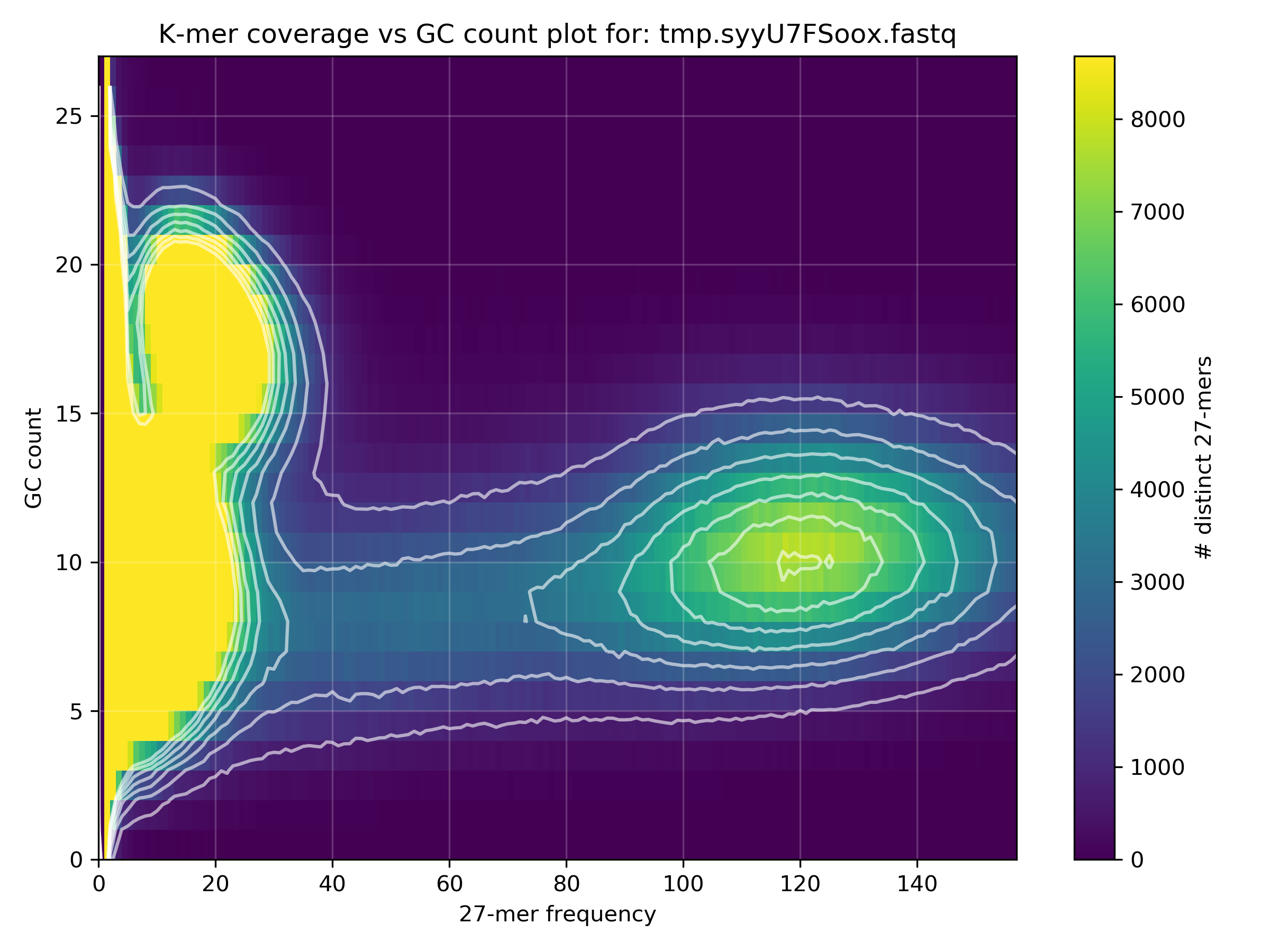

A GC content plot of SRR492065 data.

The GC content scale (Y-axis) is the absolute GC count per k-mer. The default k-mer size is 27 and therefore the y-axis is from 0 to 27. One can estimate the average GC% of a blob from this scale by multiplying the approximate GC content value by 4 (since 4 * 27 == 108 =~ 100).

Task 7.

Use kat comp to compare Enterococcus_faecalis/SRR492065_{1,2}.fastq.gz.

TMPFILE1=$(mktemp -u --suffix ".fastq")
TMPFILE2=$(mktemp -u --suffix ".fastq")
mkfifo "$TMPFILE1" && zcat "$READ1" > "$TMPFILE1" &
mkfifo "$TMPFILE2" && zcat "$READ2" > "$TMPFILE2" &
kat comp -t "$CPUS" -o "${PREFIX}_r1vr2.cmp" --density_plot "$TMPFILE1" "$TMPFILE2"
kat plot spectra-mx -x 50 -y 500000 --intersection -o "${PREFIX}_r1vr2.cmp-main.mx.spectra-mx.png" "${PREFIX}_r1vr2.cmp-main.mx"
rm "$TMPFILE1" "$TMPFILE2"

Why is there a difference in the distribution means between the two datasets?

Solution - click to expand

READ1=Enterococcus_faecalis/SRR492065_1.fastq.gz
READ2=Enterococcus_faecalis/SRR492065_2.fastq.gz
PREFIX=$(basename ${READ1%_1.*} )
TMPFILE1=$(mktemp -u --suffix ".fastq")
TMPFILE2=$(mktemp -u --suffix ".fastq")
mkfifo "$TMPFILE1" && zcat "$READ1" > "$TMPFILE1" &
mkfifo "$TMPFILE2" && zcat "$READ2" > "$TMPFILE2" &
kat comp -t "$CPUS" -o "${PREFIX}_r1vr2.cmp" --density_plot "$TMPFILE1" "$TMPFILE2"
kat plot spectra-mx -x 50 -y 500000 --intersection -o "${PREFIX}_r1vr2.cmp-main.mx.spectra-mx.png" "${PREFIX}_r1vr2.cmp-main.mx"
rm "$TMPFILE1" "$TMPFILE2"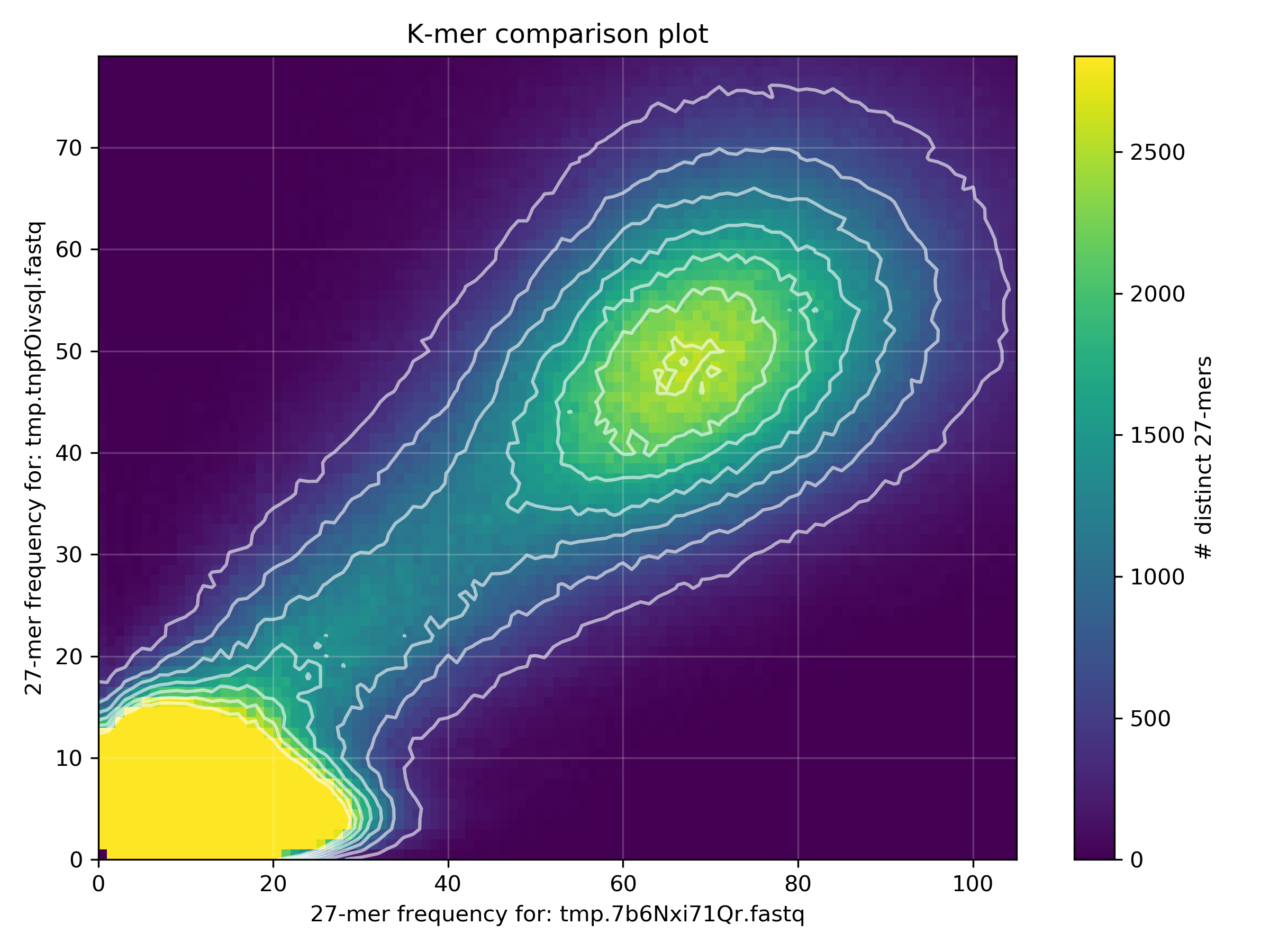

A density plot of READ1 vs READ2 in the SRR492065 data.

A spectra-mx plot of READ1 vs READ2 in the SRR492065 data.

The spectra-mx plot shows the shared content for dataset 2 (READ2) is shifted to the left and slightly higher than the shared content of dataset 1 (READ1). From the previous FastQC analyses of these files we saw that READ2 has lower read qualities than READ1. Lower quality reads mean more errors and ambiguous bases, resulting in lower k-mer frequency counts (in READ2) which shifts the mean k-mer frequency to the left.