Gene body coverage analysis in R

Per Unneberg

2023-12-21

About

This vignette describes analyses of gene body coverage and other genome assembly evaluation metrics with in R using the genecovr package. genecovr contains functionality for parsing alignment files, calculating gene body coverages, and generating simple QC metrics to assess assembly quality output. Before we start with the example analysis, we describe how genecovr represents pairwise alignments.

R setup

library(genecovr)
library(ggplot2)
library(S4Vectors)
library(tidyr)
library(rlang)

library(viridis)
library(RColorBrewer)
bw <- theme_bw(base_size = 18) %+replace%
  theme(axis.text.x = element_text(angle = 45, hjust = 1, vjust = 1))
theme_set(bw)
color_pal_4 <- brewer.pal(name = "Paired", n = 4)
psize <- 3

On object representation of pairwise sequence alignments

genecovr has functionality to read pairwise sequence alignment files and converts the pairwise alignments to genecovr::AlignmentPairs objects. An AlignmentPairs object is a subclass of the Bioconductor class S4Vectors::Pairs. A Pairs object in turn aligns two vectors along slot names first and second, and the AlignmentPairs object adds slots for the query and subject, and possibly extra slots related to additional information in the alignment file. The query and subject are GenomicRanges::GRanges objects or objects derived from the GRangesclass.

Analysing gene body coverage

In this section we analyse the mapping of a transcriptome to a non-polished and polished assembly, using example data. The entire analysis takes less than 5 minutes to execute using these datasets. The mapping results consist of two gmap files in psl format, transcripts2nonpolished.psl and transcripts2polished.psl. In addition there are fasta index files for both assemblies (nonpolished.fai and polished.fai) and for the transcriptome (transcripts.fai). The fasta indices are used to generate GenomeInfoDb::Seqinfo objects that can be used to set sequence information on the parsed output. We load the fasta indices and parse the psl files with genecovr::readPsl, storing the results in an genecovr::AlignmentPairsList for convenience.

assembly_fai_fn <- list(
  nonpol = system.file("extdata", "nonpolished.fai",
    package = "genecovr"
  ),
  pol = system.file("extdata", "polished.fai",
    package = "genecovr"
  )
)
transcripts_fai_fn <- list(
  nonpol = system.file("extdata", "transcripts.fai",
    package = "genecovr"
  ),
  pol = system.file("extdata", "transcripts.fai",
    package = "genecovr"
  )
)

assembly_sinfo <- endoapply(assembly_fai_fn, readFastaIndex)
transcripts_sinfo <- endoapply(transcripts_fai_fn, readFastaIndex)

psl_fn <- list(
  nonpol = system.file("extdata", "transcripts2nonpolished.psl",
    package = "genecovr"
  ),
  pol = system.file("extdata", "transcripts2polished.psl",
    package = "genecovr"
  )
)

apl <- AlignmentPairsList(
  lapply(names(psl_fn), function(x) {
    readPsl(psl_fn[[x]],
      seqinfo.sbjct = assembly_sinfo[[x]],
      seqinfo.query = transcripts_sinfo[[x]]
    )
  })
)
names(apl) <- names(psl_fn)

Plot ratio matches to width of alignment regions

We first plot the ratio of matches to width of alignments with respect to the transcripts.

plot(apl, aes(x = id, y = matches / query.width, fill = id), which = "violin") +
  ylim(0.8, 1) + scale_fill_viridis_d()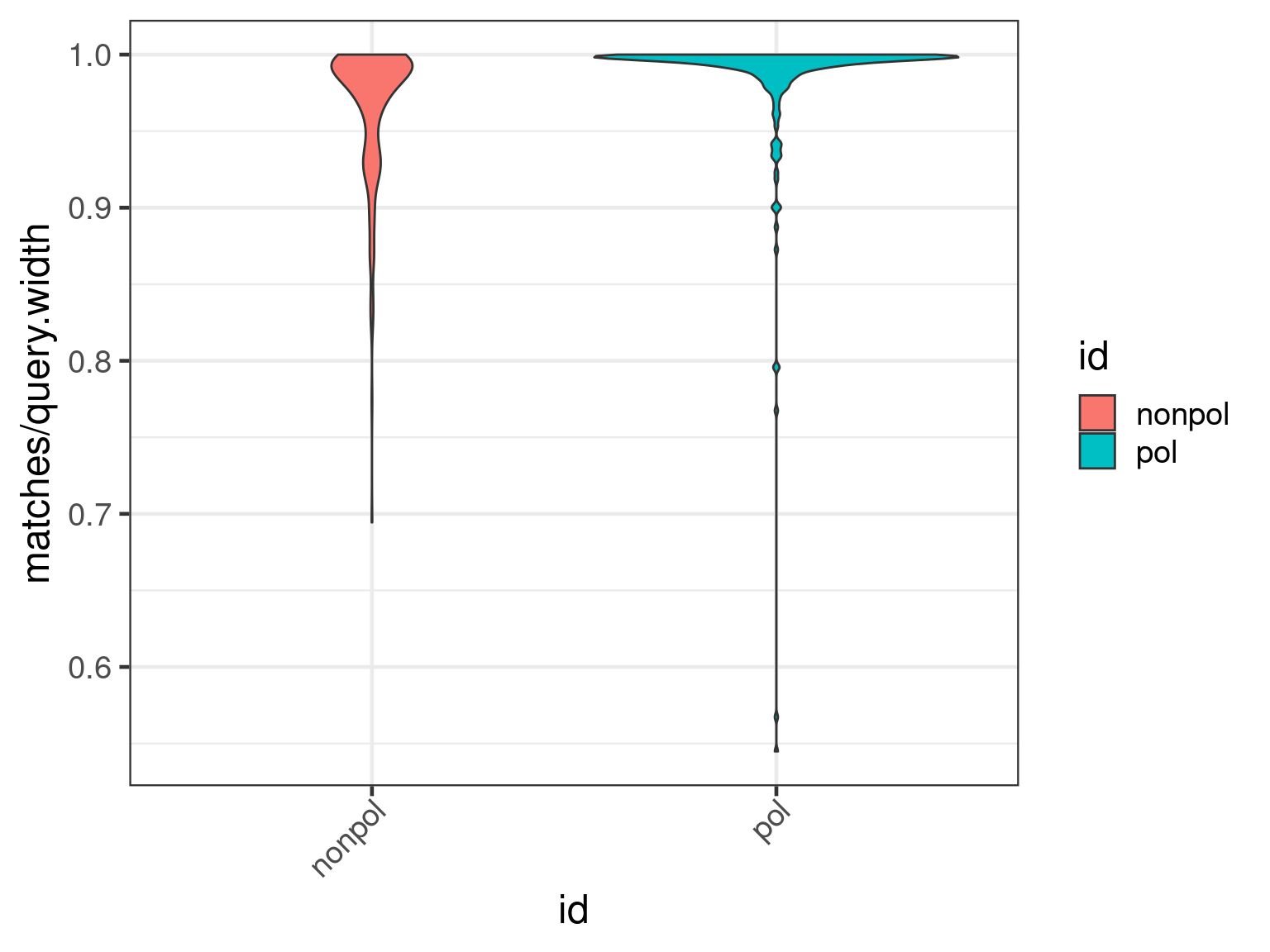

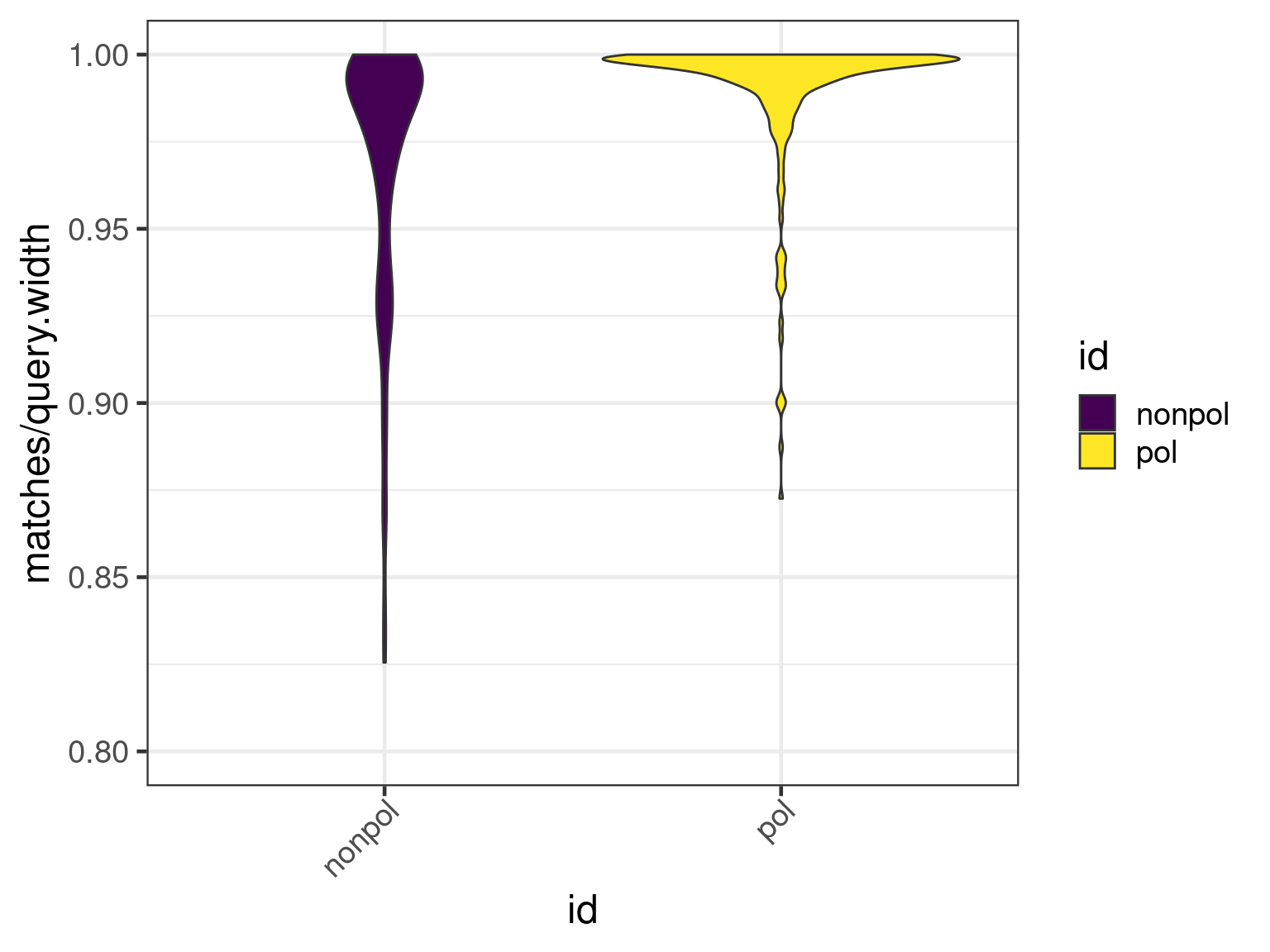
There is a clear shift to higher percentage matches in the polished assembly, as expected.

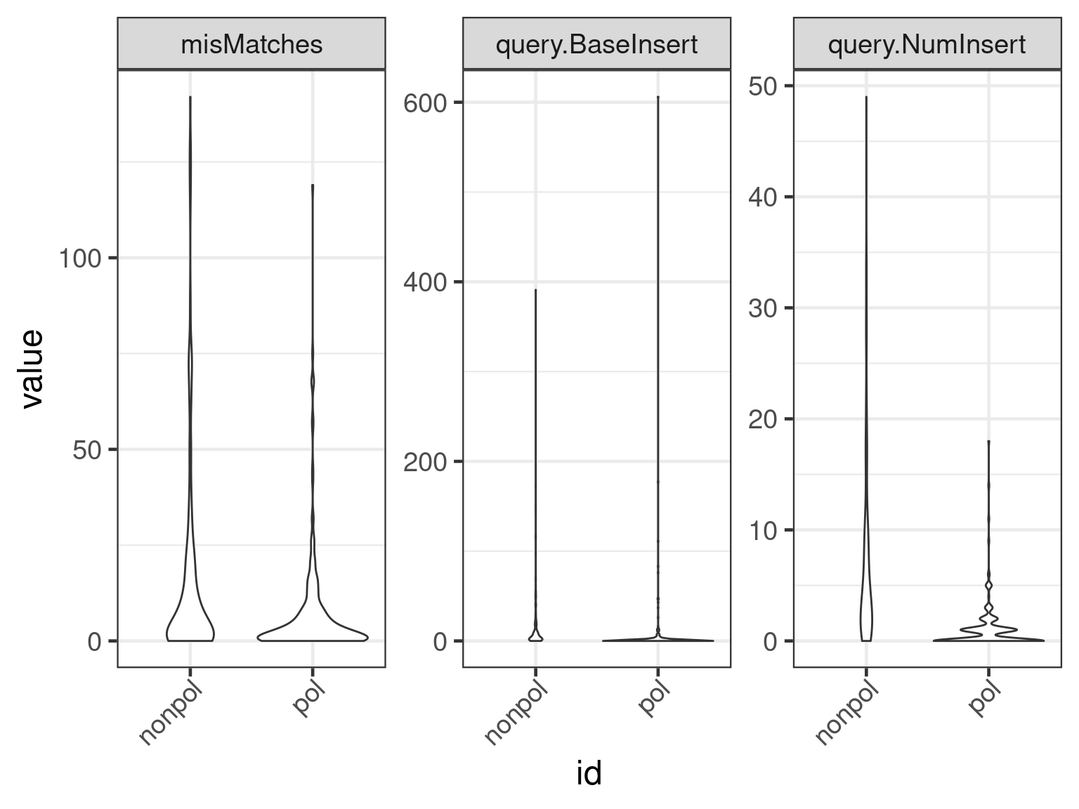
Plot summary indel and match distributions

We can also select multiple columns to plot in the genecovr::AlignmentPairsList.

cnames <- c("misMatches", "query.NumInsert", "query.BaseInsert")
plot(apl, aes(x = id, y = get_expr(enquo(cnames))), which = "violin") +
  facet_wrap(. ~ name, scales = "free")

plot(apl, aes(x = id, y = get_expr(enquo(cnames))), which = "boxplot") +
  facet_wrap(. ~ name, scales = "free")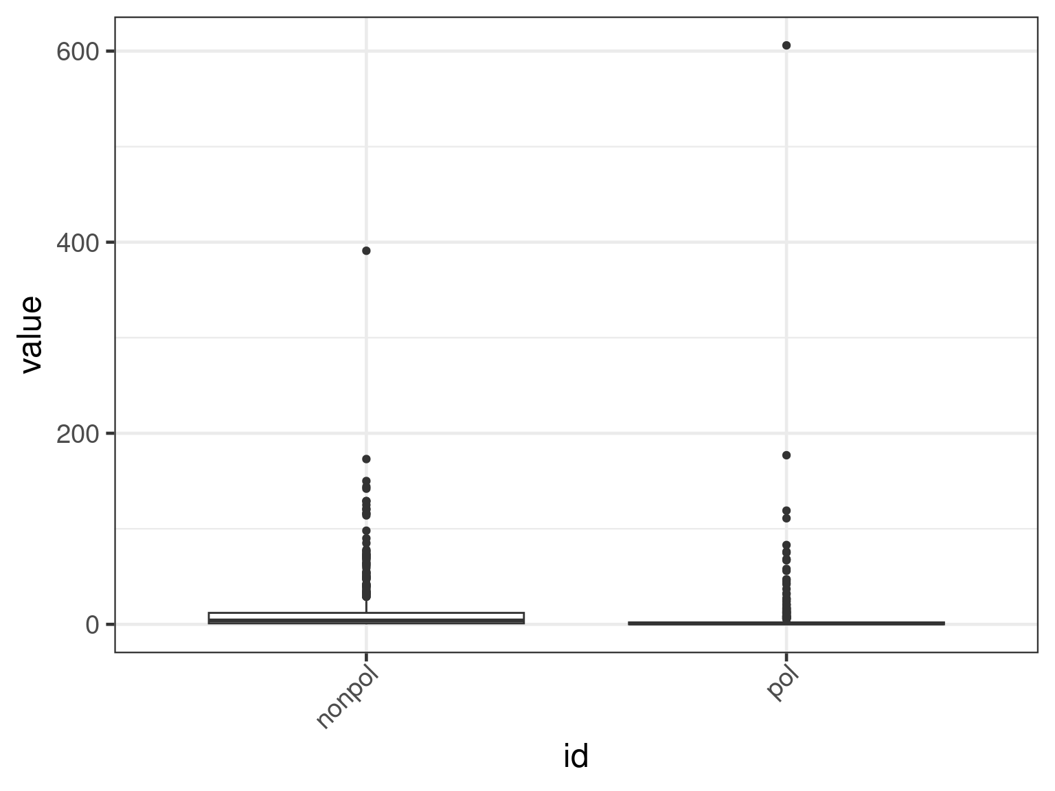

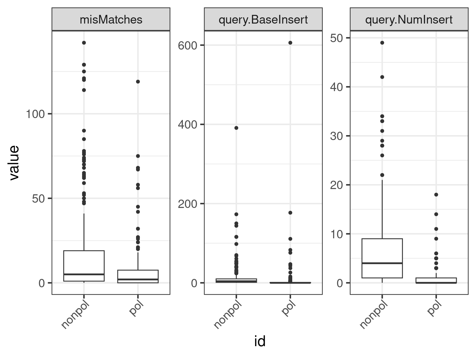
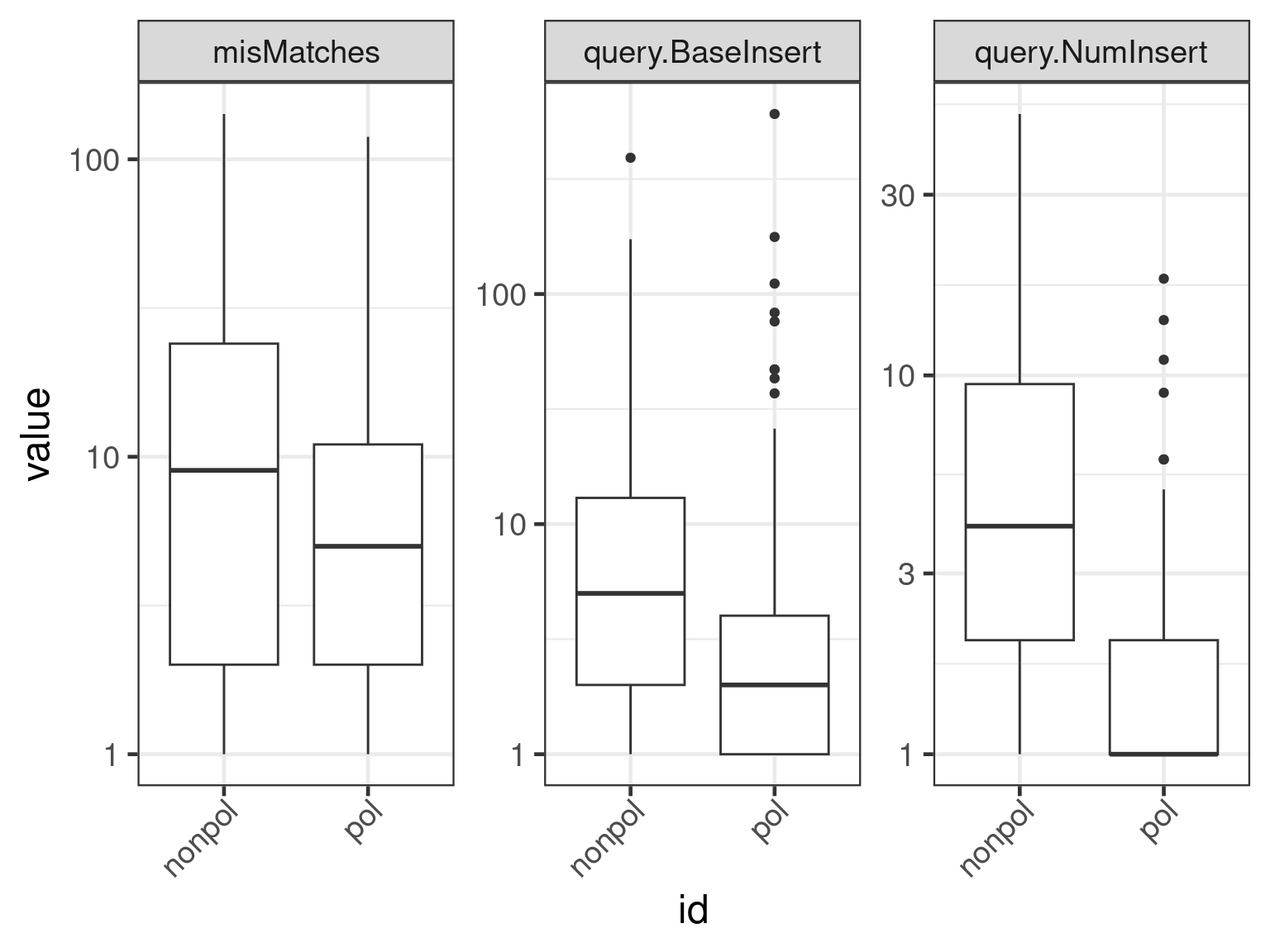
plot(apl, aes(x = id, y = get_expr(enquo(cnames))), which = "boxplot") +
  facet_wrap(. ~ name, scales = "free") + scale_y_continuous(trans = "log10")

Plot number of indels

The function genecovr::insertionSummary summarizes the number of insertions, either at the transcript level (default) or per alignment. The intuition is that as assembly quality improves, the number of indels go down.

First we show a plot with the number of insertions per alignment. A consequence of this is that as a transcript may be split in multiple alignments, the bars are of unequal height.

x <- insertionSummary(apl, reduce = FALSE)
ggplot(x, aes(id)) +
  geom_bar(aes(fill = cuts)) +
  scale_fill_viridis_d(name = "qNumInsert", begin = 1, end = 0)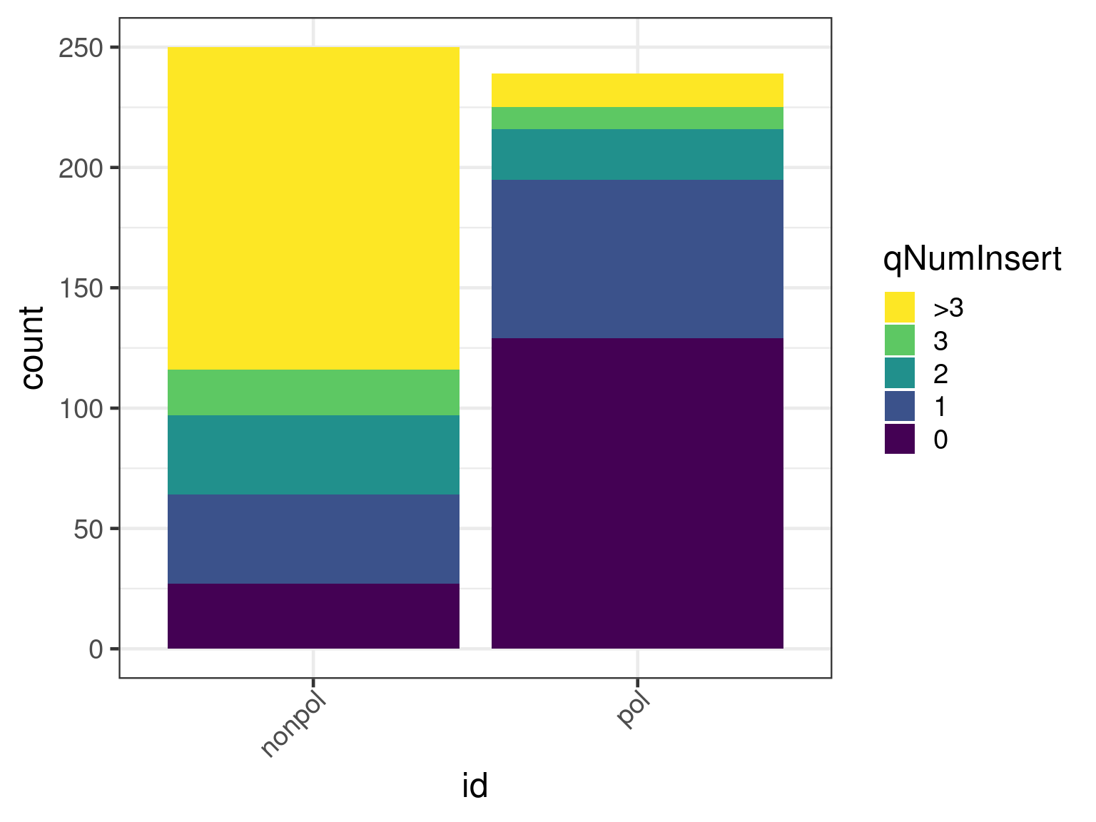

An alternative is to summarize the number of insertions over a transcript. Currently, no consideration is taken to overlapping alignments, meaning some insertions may be counted more than once. An improvement would be to use the non-overlapping set of alignments with the fewest number of insertions.

x <- insertionSummary(apl)
ggplot(x, aes(id)) +
  geom_bar(aes(fill = cuts)) +
  scale_fill_viridis_d(name = "qNumInsert", begin = 1, end = 0)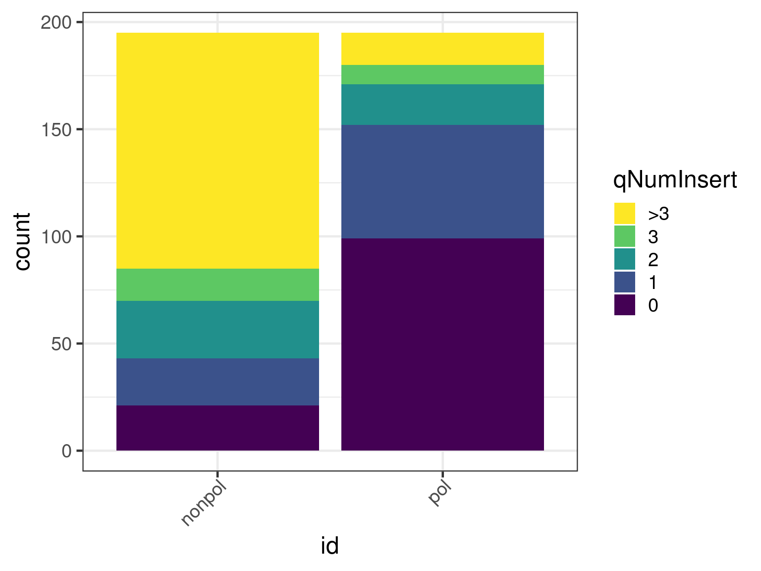

Gene body coverage

The function genecovr::geneBodyCoverage takes an AlignmentPairs object and summarizes breadth of coverage and number of subject hits per transcript.

gbc <- lapply(apl, geneBodyCoverage, min.match = 0.1)

A summary can be obtained with the genecovr::summarizeGeneBodyCoverage function. We define a range of minimum match hit cutoffs to filter out hits with too few matches in the aligned region.

min.match <- c(0.25, 0.5, 0.75, 0.9)
names(min.match) <- min.match
gbc_summary <- lapply(apl, function(x) {
  y <- do.call("rbind", lapply(min.match, function(mm) {
    summarizeGeneBodyCoverage(x, min.match = mm)
  }))
})

We combine the data

library(dplyr)
data <- dplyr::bind_rows(lapply(gbc_summary, data.frame), .id = "dataset")

and plot the resulting coverages

h <- max(data$total)
hmax <- ceiling(h / 100) * 100
ggplot(
  subset(data, min.match == 0.25),
  aes(x = min.coverage, y = count, group = dataset, color = dataset)
) +
  geom_abline(slope = 0, intercept = h) +
  geom_point(aes(shape = dataset, color = dataset), size = psize) +
  geom_line() +
  scale_color_viridis_d() +
  scale_y_continuous(breaks = c(pretty(data$count)), limits = c(0, hmax))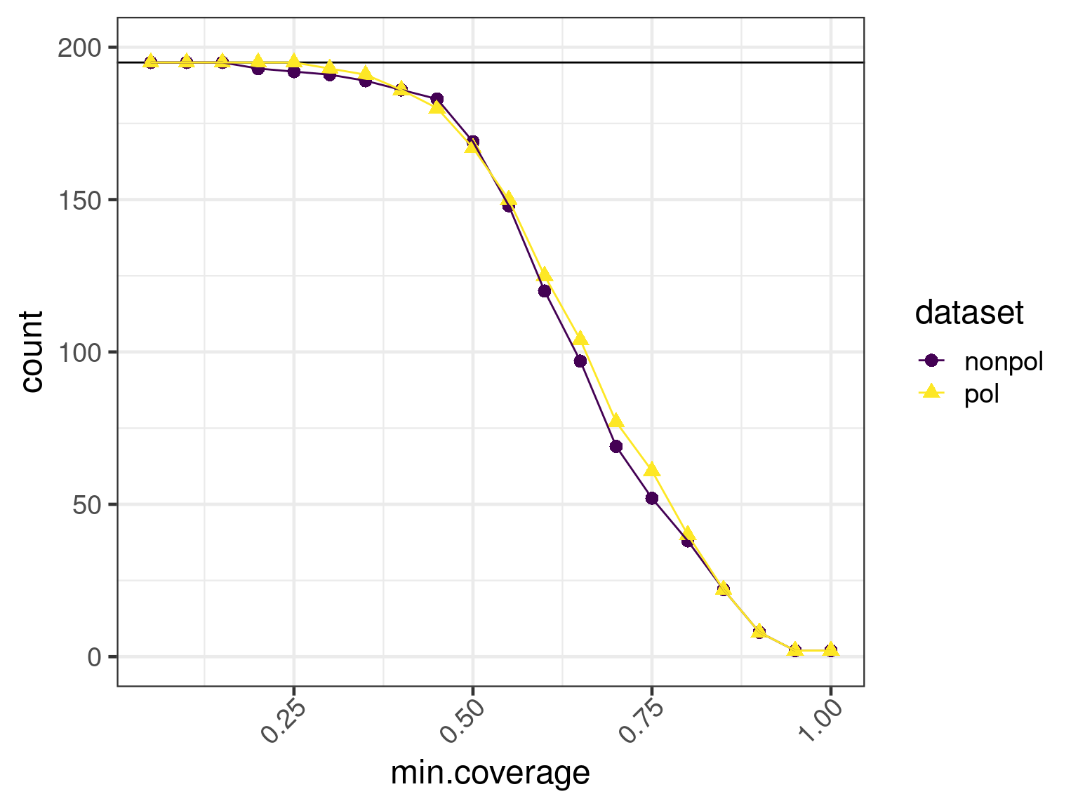

Number of contigs per transcript

A fragmented assembly will lead to more transcripts mapping to several contigs. We calculate the number of subjects by coverage cutoff with the function genecovr::countSubjectsByCoverage

data <- dplyr::bind_rows(
  lapply(
    lapply(apl, countSubjectsByCoverage),
    data.frame
  ),
  .id = "dataset"
)

and plot the results

ggplot(data = data, aes(
  x = factor(min.coverage),
  y = Freq, fill = n.subjects
)) +
  geom_bar(stat = "identity", position = position_stack()) +
  scale_fill_viridis_d(begin = 1, end = 0) +
  facet_wrap(. ~ dataset, nrow = 1, labeller = label_both)

Duplicated versus split transcripts

Transcripts that map to more than one contig could be anything from being split between the contigs to being duplicated entirely in the subjects. One way to investigate whether or not trancripts are split or duplicated is to plot the depth of coverage divided by the breadth of coverage against length-normalized coverage.

First combine the data:

data <- dplyr::bind_rows(
  lapply(
    lapply(apl, geneBodyCoverage),
    data.frame
  ),
  .id = "dataset"
)

and plot the ratio depthOfCoverage / breadthOfCoverage against length-normalized coverage

ggplot(data = data, aes(
  x = coverage, y = depthOfCoverage / breadthOfCoverage,
  color = factor(n.subjects)
)) +
  geom_point(size = psize) +
  scale_color_viridis_d(alpha = .8) +
  xlim(0, 1) +
  ylim(0, 5) +
  facet_wrap(. ~ dataset)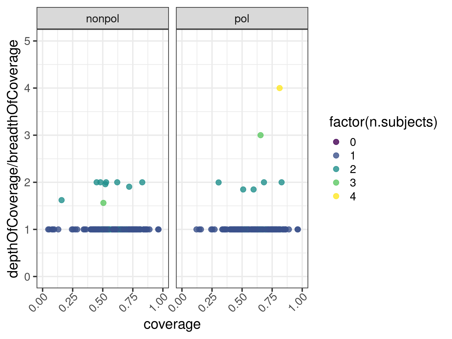

Alternatively we can make a jitter plot of the depthOfCoverage by breadthOfCoverage against number of subjects.

ggplot(
  data = subset(data, n.subjects > 1),
  aes(x = factor(dataset), y = depthOfCoverage / breadthOfCoverage)
) +
  geom_jitter(size = psize, alpha = .6) +
  facet_wrap(. ~ n.subjects)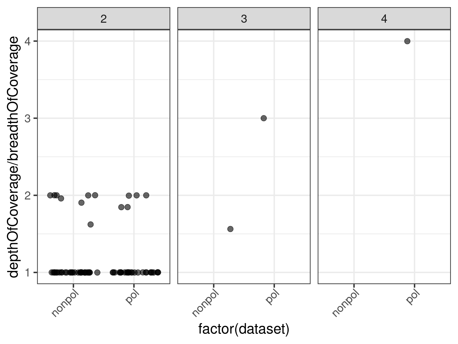

A similar picture is obtained via a histogram plot.

ggplot(
  data = subset(data, n.subjects > 1),
  aes(depthOfCoverage / breadthOfCoverage)
) +
  geom_histogram() +
  facet_grid(vars(dataset))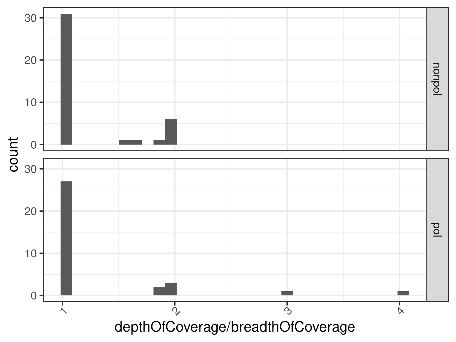

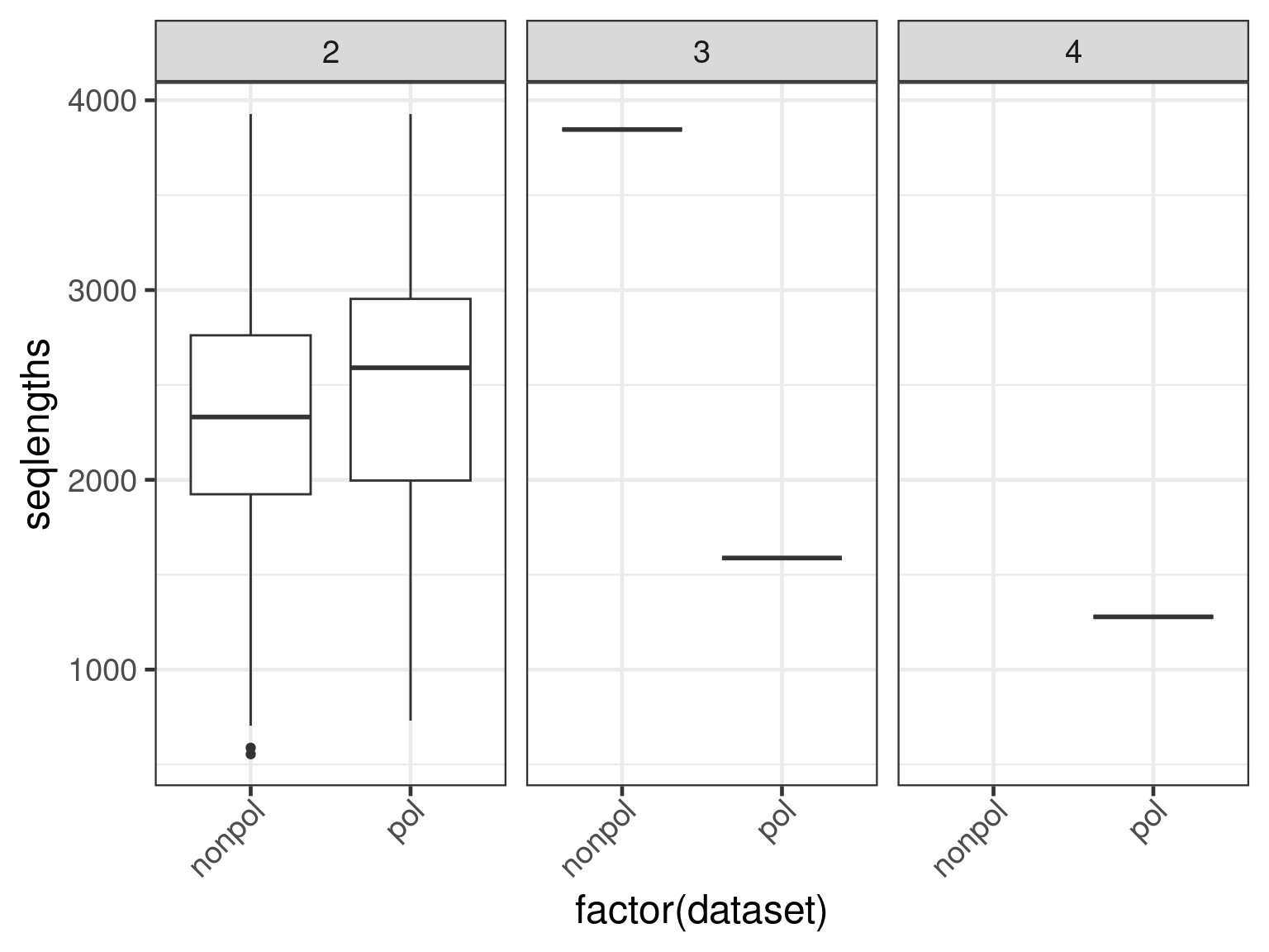
Finally, we assess whether there is a length bias in the ratio condition on the number of subjects per transcript.

ggplot(
  data = subset(data, n.subjects > 1),
  aes(x = factor(dataset), y = seqlengths)
) +
  geom_boxplot() +
  facet_grid(. ~ n.subjects)