Let’s try to build a classifier to predict obesity (Obese vs Non-obese) given our diabetes data set. To start simple:
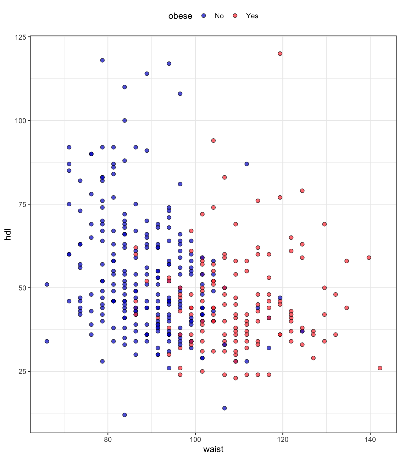
we will see how well we can predict obesity given waist and hdl variables
we will use data splitting into train, validation and test, i.e. not cross-validation with the help of splitTools() library
we will use KNN algorithm as implemented in kknn() function in library(kknn)
Reading in data
# load librarieslibrary(tidyverse)library(splitTools)library(kknn)# input datainput_diabetes <-read_csv("data/data-diabetes.csv")# clean datainch2cm <-2.54pound2kg <-0.45data_diabetes <- input_diabetes %>%mutate(height = height * inch2cm /100, height =round(height, 2)) %>%mutate(waist = waist * inch2cm) %>%mutate(weight = weight * pound2kg, weight =round(weight, 2)) %>%mutate(BMI = weight / height^2, BMI =round(BMI, 2)) %>%mutate(obese=cut(BMI, breaks =c(0, 29.9, 100), labels =c("No", "Yes"))) %>%mutate(diabetic =ifelse(glyhb >7, "Yes", "No"), diabetic =factor(diabetic, levels =c("No", "Yes"))) %>%mutate(location =factor(location)) %>%mutate(frame =factor(frame)) %>%mutate(gender =factor(gender))# select data for KNNdata_input <- data_diabetes %>%select(obese, waist, hdl) %>%na.omit()# How many obese and non-obese in our data set?data_input %>%count(obese)## # A tibble: 2 × 2## obese n## <fct> <int>## 1 No 250## 2 Yes 144# preview dataglimpse(data_input)## Rows: 394## Columns: 3## $ obese <fct> No, Yes, Yes, No, No, No, No, Yes, No, Yes, No, Yes, Yes, Yes, N…## $ waist <dbl> 73.66, 116.84, 124.46, 83.82, 111.76, 91.44, 116.84, 86.36, 86.3…## $ hdl <dbl> 56, 24, 37, 12, 28, 69, 41, 44, 49, 40, 54, 34, 36, 46, 30, 47, …data_input %>%ggplot(aes(x = waist, y = hdl, fill = obese)) +geom_point(shape=21, alpha =0.7, size =2) +theme_bw() +scale_fill_manual(values =c("blue3", "brown1")) +theme(legend.position ="top")
Splitting data
# split data into train (40%), validation (40%) and test (20%)# stratify by obeserandseed <-123set.seed(randseed)inds <-partition(data_input$obese, p =c(train =0.4, valid =0.4, test =0.2), seed = randseed)str(inds)## List of 3## $ train: int [1:158] 6 8 11 16 17 22 26 28 32 35 ...## $ valid: int [1:157] 1 3 5 7 9 10 13 14 15 24 ...## $ test : int [1:79] 2 4 12 18 19 20 21 23 27 30 ...data_train <- data_input[inds$train, ]data_valid <- data_input[inds$valid,]data_test <- data_input[inds$test, ]# check dimensions of datadata_train %>%dim()## [1] 158 3data_valid %>%dim()## [1] 157 3data_test %>%dim()## [1] 79 3# check distribution of obese and non-obesedata_train %>%group_by(obese) %>%count()## # A tibble: 2 × 2## # Groups: obese [2]## obese n## <fct> <int>## 1 No 100## 2 Yes 58data_valid %>%group_by(obese) %>%count()## # A tibble: 2 × 2## # Groups: obese [2]## obese n## <fct> <int>## 1 No 100## 2 Yes 57data_test %>%group_by(obese) %>%count()## # A tibble: 2 × 2## # Groups: obese [2]## obese n## <fct> <int>## 1 No 50## 2 Yes 29
Training KNN
# prepare parameters search spacen <-nrow(data_train)k_values <-seq(1, n-1, 2) # check every odd value of k between 1 and number of samples-1# allocate empty vector to collect overall classification rate for each kcls_rate <-rep(0, length(k_values)) for (l inseq_along(k_values)){# fit model given k value model <-kknn(obese ~., data_train, data_valid, k = k_values[l], kernel ="rectangular")# extract predicted class (predicted obesity status) cls_pred <- model$fitted.values# define actual class (actual obesity status) cls_true <- data_valid$obese# calculate overall classification rate cls_rate[l] <-sum((cls_pred == cls_true))/length(cls_pred)}
Selecting best \(k\)
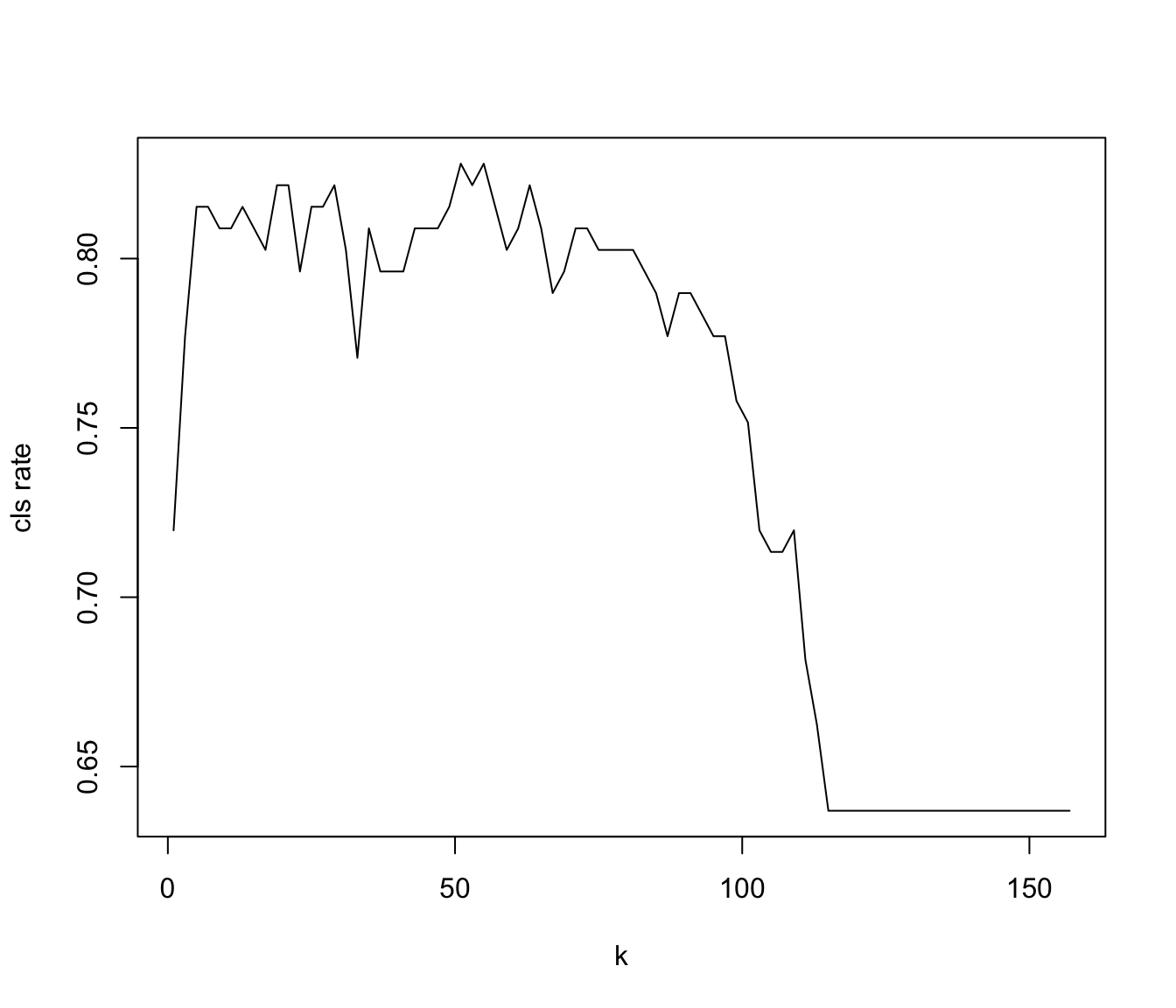
# plot classification rate as a function of kplot(k_values, cls_rate, type="l", xlab="k", ylab="cls rate")
Overall classification rate as a function of k
# For which value of k do we reach the highest classification rate?k_best <- k_values[which.max(cls_rate)]print(k_best)## [1] 51
Final model and performance on future unseen data (test data)
# How would our model perform on the future data using the optimal k?model_final <-kknn(obese ~., data_train, data_test, k=k_best, kernel ="rectangular")cls_pred <- model_final$fitted.valuescls_true <- data_test$obesecls_rate <-sum((cls_pred == cls_true))/length(cls_pred)print(cls_rate)## [1] 0.8481013