Note

These are exercises to get you started with Quarto. Refer to the official Quarto documentation for help.

By the end of this exercise, you will be able to:

Create and render a Quarto document in RStudio.
Understand the structure of a Quarto document, including the YAML header.
Add and format text using Markdown.
Include and customize code chunks.
Generate and embed visualizations.
Render Quarto documents to different formats, such as HTML and PDF reports
Set-up Quarto project

Dataset

For this exercise we will use the penguins dataset from the palmerpenguins package.

1 Introduction

Let’s start with creating your first Quarto document.

A Quarto file is a plain text file with the extension .qmd. It contains three sections: YAML header, the markdown text and code in code chunks.

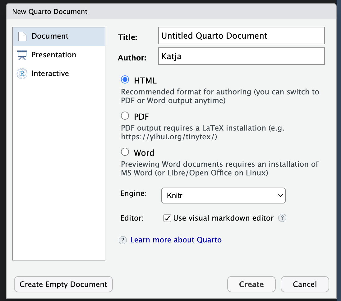
To create your own .qmd file, go to File > New File > Quarto Document.

In the Title field, give a title for your document, in that case let’s name it Untitled Quarto Document and add your name to the Author field. Next, you will select the output format for your document. By default, RStudio suggests using HTML as the output, let’s leave that default for now.

This document that you are going to work with is a Quarto notebook or R notebook. Once .qmd document is created you can set the display mode to Source or Visual (where text formatting is shown) editor.

2 YAML header

A new document is created with the following YAML.

---
title: "Untitled Quarto Document"
author: "Katja"
format: html
---

The content on the top of the Quarto document within three dashes is the YAML header. By tweaking the parameters of the YAML header we can customize the appearance and behavior of the document. It is up to the author to decide how much information needs to be entered here. Parameters in the YAML are specified in the form of key: value.

For example, you can add include title, author, subtitle, date, format… The format field specifies what type of output you want the final report to be in. Here we have specified that we want HTML format as output, which is the default output format and perhaps the most useful for scientific computing. For a complete guide to YAML metadata for HTML, see here.

YAML identation

The structure of a YAML is very particular about indentation, and errors may occur if it is not formatted correctly. If you encounter cryptic error messages about keywords in your YAML then it is worth checking the spacing of items carefully.

Change the title in the YAML header to My first Quarto Document. You can also try to add subtitle and description.

What about date parameter? Let’s use the YAML header date field to record the date we started working on the notebook.

---
title: "My first Quarto Document"
author: "Katja"
date: 2025-05-14
format: html
---

Date can also be set as last-modified which means it is automatically updated whenever the document is rendered. The date format is adjusted by setting date-format: “YYYY-MMM-DD”.

---
title: "My first Quarto Document"
author: "Katja"
date: last-modified
date-format: “YYYY-MMM-DD"
format: html
---

You can also use the today option.

Add the following to the YAML header: date: today

Now you have generated document with no content, so rendering it, would not result in very interesting output, i.e. rendering will produce a blank html document. Let’s add a little bit of content to the document, starting with some basic markdown text.

Add the text from below into your Quarto document (including an empty line between the YAML header and the text):

This is my first Quarto document!

# This is a header

This is where I will soon add some *code* related to the first header.

Before you render the document into HTML let’s check what rendering is and how it works.

Rendering

When you render the document, Quarto sends the .qmd file to knitr, which executes all of the code chunks and creates a new markdown (.md) document which includes the code and its output. The markdown file generated by knitr is then processed by pandoc, which is responsible for creating the finished file. The advantage of this two step workflow is that you can create a very wide range of output formats (HTML, PDF, MS Word…).

Now is your turn to render the existing document.

Click the Render button, which you can find either in the toolbar above the document (button with a blue arrow) or under the “File” tab
The output will open in a new tab in your web browser (Chrome, Safari, Firefox etc.)

3 Markdown text

Markdown is a plain text format that is designed to be easy to write, and even more importantly, easy to read. Quarto is based on Pandoc and uses its variation of markdown.

Markdown text is useful to introduce your content and explain your code.

3.1 Text formatting

This *italic text* becomes italic text.
This **bold text** becomes bold text. Subscript written like this H~2~O renders as H₂O.
Superscript written like this 2^10^ renders as 2¹⁰. This code format becomes code.

3.2 Headings

# Level 1 heading
## Level 2 heading  
### Level 3 heading  
#### Level 4 heading

3.3 Lists

-   Bulleted list item 1

-   Item 2

    -   Item 2a

    -   Item 2b

Bulleted list item 1
Item 2
- Item 2a
- Item 2b

1.  Numbered list item 1

2.  Item 2.
    The numbers are incremented automatically in the output.

Numbered list item 1
Item 2. The numbers are incremented automatically in the output.

3.4 Links

Links can be created using <https://quarto.org> which renders like https://quarto.org or using [this](https://quarto.org) which renders like this this.

3.5 Figures

The figures in a Quarto document can be embedded (e.g., a PNG or JPEG file) or generated as a result of a code chunk.

Images can be displayed from a relative local location using ![These are Palmer penguins](./images/lter_penguins.png).

By default, the image is displayed at full scale or until it fills the display width. The image dimension can be adjusted ![These are Palmer penguins](./images/lter_penguins.png){width=40%}.

RStudio - Figure / Image

To embed an image from an external file, you can use the Insert menu in the Visual Editor in RStudio and select Figure / Image. This will open a menu where you can browse to the image you want to insert as well as add alternative text or caption to it and adjust its size. In the Visual Editor you can also simply paste an image from your clipboard into your document and RStudio will place a copy of that image in your project folder.

In your Quarto document, rename first header from # This is a header to Introduction. Replace existing markdown text under the first header with some text related to Quarto notebook, for example This is my first Quarto document. The goal is to build a Quarto report using different Quarto features. To existing markdown text add link to Quarto webpage. Save the document.
Create another header (level 1), Palmer penguins. Find some information about palmerpenguins dataset, and add markdown text under the second header. Add link to the palmerpenguins R package. Finally, download image of the three penguins and insert image to the document. Save the document and render.

3.6 Tables

Similar to figures, you can include two types of tables in a Quarto document. They can be markdown tables that you create directly in your Quarto document (using the Insert Table menu in the Visual Editor in RStudio) or they can be tables generated as a result of a code chunk. Here is an example of markdown table known as a pipe table.

| First Header | Second Header |
|--------------|---------------|
| Content Cell | Content Cell  |
| Content Cell | Content Cell  |

First Header	Second Header
Content Cell	Content Cell
Content Cell	Content Cell

4 Code

Code blocks are called chunks. Chunks refer to sections in the document where you can write and execute code. These chunks are enclosed by three backticks followed by the name of the language you are using (e.g., r for R code). Code chunks can be included in three ways:

Keyboard commands: ⌃Ctrl + Alt + I (Windows) or Cmd + Option + I (Mac)
RStudio: Clicking the Insert button in the toolbar (top right) in the Visual Editor, choose Executable Cell
Manually typing the chunk delimiters

Block code formatted as such:

```{r}
str(penguins)
```

renders like this:

str(penguins)

tibble [344 × 8] (S3: tbl_df/tbl/data.frame)
 $ species          : Factor w/ 3 levels "Adelie","Chinstrap",..: 1 1 1 1 1 1 1 1 1 1 ...
 $ island           : Factor w/ 3 levels "Biscoe","Dream",..: 3 3 3 3 3 3 3 3 3 3 ...
 $ bill_length_mm   : num [1:344] 39.1 39.5 40.3 NA 36.7 39.3 38.9 39.2 34.1 42 ...
 $ bill_depth_mm    : num [1:344] 18.7 17.4 18 NA 19.3 20.6 17.8 19.6 18.1 20.2 ...
 $ flipper_length_mm: int [1:344] 181 186 195 NA 193 190 181 195 193 190 ...
 $ body_mass_g      : int [1:344] 3750 3800 3250 NA 3450 3650 3625 4675 3475 4250 ...
 $ sex              : Factor w/ 2 levels "female","male": 2 1 1 NA 1 2 1 2 NA NA ...
 $ year             : int [1:344] 2007 2007 2007 2007 2007 2007 2007 2007 2007 2007 ...

The chunk is executed when this document is rendered. In the above example, the rendered output has two chunks; input and output chunks.

The behaviour of code chunks can be adjusted using chunk parameters or execution options. For example you can specify if your code block is executed, what results are inserted in the rendered report, the width and height of generated figures. Chunk options are in YAML format and identified by #| at the beginning of the line.

In this chunk we set eval: false which will prevent chunk from being executed, while setting eval: true (default), executes the chunk.

```{r}
#| eval: false

ggplot(penguins, aes(x = sex, fill = species)) +
  geom_bar(alpha = 0.8) +
  scale_fill_manual(values = c("darkorange","purple","cyan4"), 
                    guide = FALSE) +
  theme_minimal() +
  facet_wrap(~species, ncol = 1) +
  coord_flip()
```

Using echo: false prevents the code from that chunk from being displayed. Using output: false hides the output from that chunk.

Here are some of execution options:

Chunk option	Effect
`echo`	Include the chunk code in the output.
`eval`	Evaluate the code chunk.
`output`	Include the results of executing the code in the output.
`warning`	Include warnings in the output.
`error`	Include errors in the output (note that this implies that errors executing code will not halt processing of the document).
`include`	Prevent both code and output from being included.

Let’s go back to your Quarto notebook. Under the header Palmer penguins create a new heading (level 2) and name it Prepare dataset. Add the chunk below to your document.

```{r}
#| message: false
library(palmerpenguins)
library(ggplot2)
```

We created r chunk to load necessary r libraries, with message: false we prevent messages that are generated by code from appearing in the rendered report.

R packages

It is best practice to avoid installing packages directly within a Quarto document, as this would cause the installation to be repeated every time the document is rendered. Instead, install the packages in your terminal or within RStudio to keep your Quarto document clean.

Add another chunk to your document. Save the document, render it and check what happens.

```{r}
#| label: penguin data
#| echo: false
str(penguins)
```

Notice how we no longer see the code itself, just the output? This is because the echo option specifies just that: whether we see the code or not.

Check what happens if you change echo: false to eval: false. Now the code in the code chunk is not run but the code itself is shown in the rendered document.

4.1 R plots

If you include a code chunk that generates a figure (e.g., includes a ggplot() call), the resulting figure will be automatically included in your Quarto document.

R Plots can be plotted like below:

```{r}
#| fig-height: 6
#| fig-width: 6

ggplot(penguins, aes(x = sex, fill = species)) +
  geom_bar(alpha = 0.8) +
  scale_fill_manual(values = c("darkorange","purple","cyan4"), 
                    guide = FALSE) +
  theme_minimal() +
  facet_wrap(~species, ncol = 1) +
  coord_flip()
```

Create new header (level 1), named it Data visualization. Insert new r chunk where you will generate r plot using palmerpenguins dataset that we loaded in the previous step. Similar to the example above create a barplot where penguin counts for each species and island are shown. Specify executions options similar to the example above. Render the document.

Solution

```{r}
#| echo: false
#| fig-height: 6
#| fig-width: 6

ggplot(penguins, aes(x = island, fill = species)) +
  geom_bar(alpha = 0.8) +
  scale_fill_manual(values = c("darkorange","purple","cyan4"), 
                    guide = FALSE) +
  theme_minimal() +
  facet_wrap(~species, ncol = 1) +
  coord_flip()
```

There are two chunk options related to figure sizes: fig-width and fig-height (expressed in inches). These allow you to experiment with your figures and make them look the way you want.

Modify these two parametrs, render the document and observe changes.

You can also add captions and their location using the fig-cap and cap-location code chunk options respectively.

Add a suitable caption and caption location (options: top, bottom, margin) to the figure and render.

4.1.1 Cross-references

A convenient way to be able to refer to figures in text is by adding a figure label, which will automatically add a figure number before your caption.

Add a suitable label to the plot generated above, e.g. label: fig-islands_by_penguins to the chunk options, then render the document again.

Notice that the figure now has a number before the caption. Importantly, the label must start with fig- prefix for the numbering and cross-referencing to work. Cross-references use the @ symbol and the corresponding label.

You can thus write some markdown outside of a code chunk and refer to e.g. @fig-islands_by_penguins, as per the example here. Try this out by adding the following to your document:

A plot of penguin count for each species on all islands is shown in @fig-islands_by_penguins.

4.1.2 Subfigures

Sometimes you want to show multiple (sub) figures, and using Quarto you can create them without using a plotting library such as cowplot. This is possible with fig-subcap: chunk option.

For example:

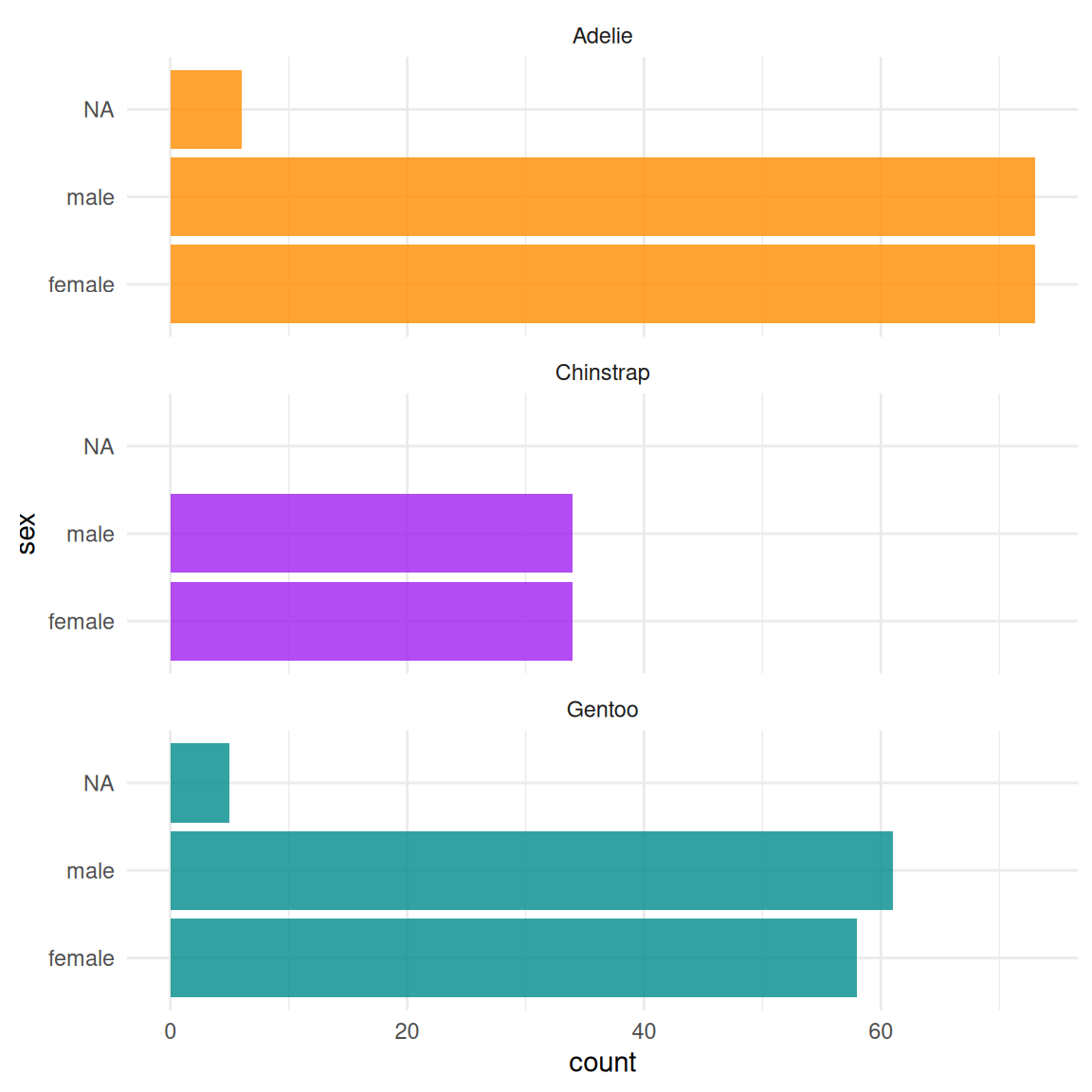
#| fig-subcap:
#|     - Penguin count for each species of each sex
#|     - Penguin count for each species on all islands

The layout of subfigures is controlled using the layout-ncol chunk option. To put multiple plots in a single row, set the layout-ncol to 2 for two plots, 3 for three plots, etc. This effectively sets out-width to “50%” for each of your plots if layout-ncol is 2, “33%” if layout-ncol is 3, etc. Depending on what you are trying to illustrate (e.g., show data or show plot variations), you might also tweak fig-width.

Create a new chunk and copy codes from steps above to obtain two figures. Set the fig-subcap: and layout-ncol: options and render the document.

4.2 Tables

Like mentioned earlier, two types of tables can be included in a Quarto document. Example below demonstrates table generated as a result of a code chunk. In order for a table to be cross-referenceable, its label must start with the tbl- prefix.

```{r}
#| label: tbl-penguins
#| tbl-cap: Palmer penguins bill length, flipper length and body mass.
#| tbl-cap-location: margin

knitr::kable(
    penguins[1:10, c("species", "bill_length_mm", "flipper_length_mm", "body_mass_g")],
    col.names = c("Species", "Bill length (mm)", "Flipper length (mm)", "Body mass (g)")
)
```

Add this code chunk to your document and render it.
Change tbl-cap-location: to top, render and observe what happens.
Under the chunk where you just generated the table, write some markdown text and refer to the table using cross-referencing.

5 Document options

Up to this point, we have mainly focused on chunk-level settings that apply only within the specific chunk they are used in. However, many of these options can also be applied globally affecting the entire document. There are also some options specifically for tailoring the document as a whole, regardless of chunk content.

When we created Quarto notebook we already applied some global options, such as title, author, date, format.

5.1 Table of contents

To make it easier for readers to navigate your document, you can use a table of contents. You just have to specify it using the toc in the YAML header. This is how the header would look like:

---
title: "My first Quarto Document"
author: "Katja"
date: last-modified
date-format: “YYYY-MMM-DD"
format: html
toc: true
---

To specify the number of section levels to include in the table of contents toc-depth option can be used. Position of the table of contents can be set-up using the toc-location. The HTML format by default floats the table of contents to the right. You can alternatively position it at the left, or in the body. You can also customize the title used for the table of contents using the toc-title option, for example: toc-title: Contents.

Add toc, toc-depth and toc-location to your document and render it.

5.2 Section numbering

This is another feature that can help browsing your document efficiently. It is very straightforward, you just need to specify number-sections: true in your YAML header. To specify the deepest level of heading to add numbers to (by default all headings are numbered) use the number-depth option.

5.3 Code folding

code-fold is one of the global options that are specified nested inside the format option, like so:

format:
  html:
    code-fold: true

Add the code-fold option to your document and render it.

You will see that Code button is generated and if you click on it chunk containing code will open. You can also use the code-summary chunk option to specify a different text to show with the folded code instead of the default Code, e.g. code-summary: Show the code.

format:
  html:
    code-fold: true
    code-summary: "Show the code"

Add the code-fold and code-summary options to your document and render it.

You can also add the code-tools option, which will add a drop-down menu to toggle visibility of all code as well as the ability to view the source of the document.

Add the code-tools: true to your document and render it.

6 Quarto project

So far, the output formats we have discussed and you have worked on have been single documents. We can also have a project composed of multiple documents and document types. In this case, the files are organised in a directory and the configuration is defined in _quarto.yml. This will be referred to as the config file. Think of this as a shared YAML metadata file for all of the documents. In addition, an index.qmd file defines the home page.

For a website, the minimal config looks like this:

project:
  type: website

And for a book:

project:
  type: book

Then running quarto render renders the output into a directory named _site. The output can be changed, for example, to docs for GitHub Pages.

project:
  type: website
  output_dir: docs

The output format by default is HTML. This can be changed or modified by adding format to the config file or to individual qmd files. The parameters defined in the config file will be shared by all other qmd files.

To create a project in RStudio, go to File > New Project , then select directory and then a project type such as website, blog or book. Try creating one based on what interests you. Website and blog documentation is here and books are here.

To read more about project, see here.