library(tidymodels)

tidymodels_prefer()
theme_set(theme_bw())
options(pillar.advice = FALSE, pillar.min_title_chars = Inf)

data(cells, package = "modeldata")
cells$case <- NULL

set.seed(123)
cell_split <- initial_split(cells, prop = 0.8, strata = class)
cell_tr <- training(cell_split)
cell_te <- testing(cell_split)0.1 The Data
0.2 Logistic Regresion
How do you fit a logistic model in R?
How many different ways can you think of?
. . .
glmfor generalized linear model (e.g. logistic regression)glmnetfor regularized regressionkerasfor regression using TensorFlowstanfor Bayesian regressionsparkfor large data sets
. . .
These all have the same model equation.
0.3 To specify a model
. . .
- Choose a model type
- Specify an engine
- Set the mode
0.4 To specify a model - choose a model type
logistic_reg()
#> Logistic Regression Model Specification (classification)
#>
#> Computational engine: glm
. . .
A different model type (= different equation)
. . .
rand_forest()
#> Random Forest Model Specification (unknown mode)
#>
#> Computational engine: ranger
Models have default engines
0.5 To specify a model
- Choose a model type
- Specify an engine
- Set the mode
0.6 To specify a model - set the engine
logistic_reg() %>%
  set_engine("glmnet")
#> Logistic Regression Model Specification (classification)
#>
#> Computational engine: glmnet
0.7 To specify a model - set the engine
logistic_reg() %>%
  set_engine("stan")
#> Logistic Regression Model Specification (classification)
#>
#> Computational engine: stan
0.8 To specify a model
- Choose a model type
- Specify an engine
- Set the mode
0.9 To specify a model - set the mode
decision_tree()
#> Decision Tree Model Specification (unknown mode)
#>
#> Computational engine: rpart
0.10 To specify a model - set the mode
decision_tree() %>%
  set_mode("classification")
#> Decision Tree Model Specification (classification)
#>
#> Computational engine: rpart
. . .
Other modes are “regression” and “censored regresion”.
. . .
All available models are listed at https://www.tidymodels.org/find/parsnip/
0.11
0.12 Models we’ll be using today
- Logistic regression
- Decision trees
0.13 A single predictor

0.14 Logistic regression - a single predictor

0.15 Logistic regression - a single predictor

- Outcome modeled as linear combination of predictors:
\(log\left(\frac{\pi}{1-\pi}\right) = \beta_0 + \beta_1x + \epsilon\)
- Find a line that maximizes the binomial (log-)likelihood function.
0.16 Decision trees - a single predictor

0.17 Decision trees - a single predictor

Series of splits or if/then statements based on predictors
First the tree grows until some condition is met (maximum depth, no more data)
Then the tree is pruned to reduce its complexity
0.18 Decision trees - a single predictor


0.19 All models are wrong, but some are useful!
0.19.1 Logistic regression

0.19.2 Decision trees

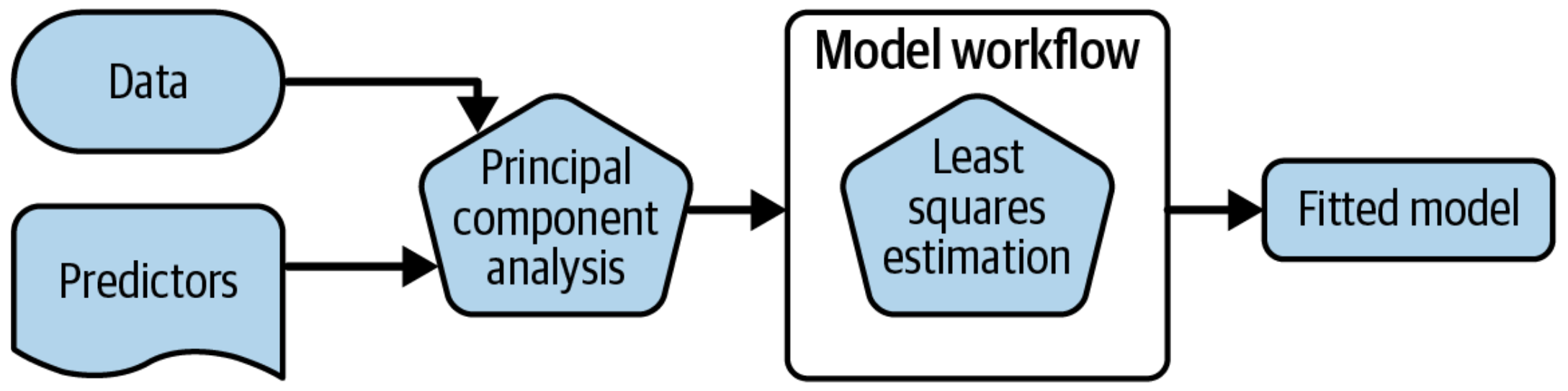
1 A model workflow
1.1 Workflows bind preprocessors and models
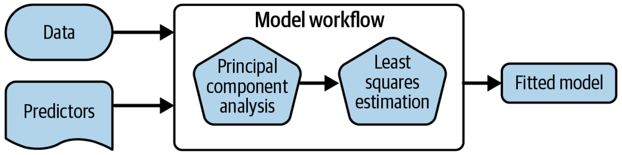
Explain that PCA that is a preprocessor / dimensionality reduction, used to decorrelate data
1.2 What is wrong with this?
1.3 Why a workflow()?
. . .
- Workflows handle new data better than base R tools in terms of new factor levels
. . .
- You can use other preprocessors besides formulas (more on feature engineering)
. . .
- They can help organize your work when working with multiple models
. . .
- Most importantly, a workflow captures the entire modeling process:
fit()andpredict()apply to the preprocessing steps in addition to the actual model fit
Two ways workflows handle levels better than base R:
Enforces that new levels are not allowed at prediction time (this is an optional check that can be turned off)
Restores missing levels that were present at fit time, but happen to be missing at prediction time (like, if your “new” data just doesn’t have an instance of that level)
1.4 A model workflow
tree_spec <-
  decision_tree() %>%
  set_mode("classification")

tree_spec %>%
  fit(class ~ ., data = cell_tr)
#> parsnip model object
#>
#> n= 1615
#>
#> node), split, n, loss, yval, (yprob)
#>       * denotes terminal node
#>
#>   1) root 1615 575 PS (0.64396285 0.35603715)
#>     2) total_inten_ch_2< 41713.5 687  40 PS (0.94177584 0.05822416) *
#>     3) total_inten_ch_2>=41713.5 928 393 WS (0.42349138 0.57650862)
#>       6) fiber_width_ch_1< 11.35657 427 160 PS (0.62529274 0.37470726)
#>        12) var_inten_ch_1< 199.704 382 122 PS (0.68062827 0.31937173)
#>          24) kurt_inten_ch_1>=-0.3456671 270  62 PS (0.77037037 0.22962963) *
#>          25) kurt_inten_ch_1< -0.3456671 112  52 WS (0.46428571 0.53571429)
#>            50) total_inten_ch_1< 13594 31   6 PS (0.80645161 0.19354839) *
#>            51) total_inten_ch_1>=13594 81  27 WS (0.33333333 0.66666667)
#>             102) diff_inten_density_ch_4>=190.8823 7   0 PS (1.00000000 0.00000000) *
#>             103) diff_inten_density_ch_4< 190.8823 74  20 WS (0.27027027 0.72972973) *
#>        13) var_inten_ch_1>=199.704 45   7 WS (0.15555556 0.84444444) *
#>       7) fiber_width_ch_1>=11.35657 501 126 WS (0.25149701 0.74850299)
#>        14) eq_ellipse_oblate_vol_ch_1>=1673.942 35  12 PS (0.65714286 0.34285714) *
#>        15) eq_ellipse_oblate_vol_ch_1< 1673.942 466 103 WS (0.22103004 0.77896996) *
1.5 A model workflow
tree_spec <-
  decision_tree() %>%
  set_mode("classification")

workflow() %>%
  add_formula(class ~ .) %>%
  add_model(tree_spec) %>%
  fit(data = cell_tr)
#> ══ Workflow [trained] ══════════════════════════════════════════════════════════
#> Preprocessor: Formula
#> Model: decision_tree()
#>
#> ── Preprocessor ────────────────────────────────────────────────────────────────
#> class ~ .
#>
#> ── Model ───────────────────────────────────────────────────────────────────────
#> n= 1615
#>
#> node), split, n, loss, yval, (yprob)
#>       * denotes terminal node
#>
#>   1) root 1615 575 PS (0.64396285 0.35603715)
#>     2) total_inten_ch_2< 41713.5 687  40 PS (0.94177584 0.05822416) *
#>     3) total_inten_ch_2>=41713.5 928 393 WS (0.42349138 0.57650862)
#>       6) fiber_width_ch_1< 11.35657 427 160 PS (0.62529274 0.37470726)
#>        12) var_inten_ch_1< 199.704 382 122 PS (0.68062827 0.31937173)
#>          24) kurt_inten_ch_1>=-0.3456671 270  62 PS (0.77037037 0.22962963) *
#>          25) kurt_inten_ch_1< -0.3456671 112  52 WS (0.46428571 0.53571429)
#>            50) total_inten_ch_1< 13594 31   6 PS (0.80645161 0.19354839) *
#>            51) total_inten_ch_1>=13594 81  27 WS (0.33333333 0.66666667)
#>             102) diff_inten_density_ch_4>=190.8823 7   0 PS (1.00000000 0.00000000) *
#>             103) diff_inten_density_ch_4< 190.8823 74  20 WS (0.27027027 0.72972973) *
#>        13) var_inten_ch_1>=199.704 45   7 WS (0.15555556 0.84444444) *
#>       7) fiber_width_ch_1>=11.35657 501 126 WS (0.25149701 0.74850299)
#>        14) eq_ellipse_oblate_vol_ch_1>=1673.942 35  12 PS (0.65714286 0.34285714) *
#>        15) eq_ellipse_oblate_vol_ch_1< 1673.942 466 103 WS (0.22103004 0.77896996) *
1.6 A model workflow
tree_spec <-
  decision_tree() %>%
  set_mode("classification")

workflow(class ~ ., tree_spec) %>%
  fit(data = cell_tr)
#> ══ Workflow [trained] ══════════════════════════════════════════════════════════
#> Preprocessor: Formula
#> Model: decision_tree()
#>
#> ── Preprocessor ────────────────────────────────────────────────────────────────
#> class ~ .
#>
#> ── Model ───────────────────────────────────────────────────────────────────────
#> n= 1615
#>
#> node), split, n, loss, yval, (yprob)
#>       * denotes terminal node
#>
#>   1) root 1615 575 PS (0.64396285 0.35603715)
#>     2) total_inten_ch_2< 41713.5 687  40 PS (0.94177584 0.05822416) *
#>     3) total_inten_ch_2>=41713.5 928 393 WS (0.42349138 0.57650862)
#>       6) fiber_width_ch_1< 11.35657 427 160 PS (0.62529274 0.37470726)
#>        12) var_inten_ch_1< 199.704 382 122 PS (0.68062827 0.31937173)
#>          24) kurt_inten_ch_1>=-0.3456671 270  62 PS (0.77037037 0.22962963) *
#>          25) kurt_inten_ch_1< -0.3456671 112  52 WS (0.46428571 0.53571429)
#>            50) total_inten_ch_1< 13594 31   6 PS (0.80645161 0.19354839) *
#>            51) total_inten_ch_1>=13594 81  27 WS (0.33333333 0.66666667)
#>             102) diff_inten_density_ch_4>=190.8823 7   0 PS (1.00000000 0.00000000) *
#>             103) diff_inten_density_ch_4< 190.8823 74  20 WS (0.27027027 0.72972973) *
#>        13) var_inten_ch_1>=199.704 45   7 WS (0.15555556 0.84444444) *
#>       7) fiber_width_ch_1>=11.35657 501 126 WS (0.25149701 0.74850299)
#>        14) eq_ellipse_oblate_vol_ch_1>=1673.942 35  12 PS (0.65714286 0.34285714) *
#>        15) eq_ellipse_oblate_vol_ch_1< 1673.942 466 103 WS (0.22103004 0.77896996) *
1.7 Predict with your model
How do you use your new tree_fit model?
tree_spec <-
  decision_tree() %>%
  set_mode("classification")

tree_fit <-
  workflow(class ~ ., tree_spec) %>%
  fit(data = cell_tr)

predict(tree_fit, cell_te %>% slice(1:6), type = "prob")| .pred_PS | .pred_WS |
|---|---|
| 0.9417758 | 0.0582242 |
| 0.2210300 | 0.7789700 |
| 0.2210300 | 0.7789700 |
| 0.9417758 | 0.0582242 |
| 0.2210300 | 0.7789700 |
| 0.9417758 | 0.0582242 |
2 The tidymodels prediction guarantee!
. . .
- The predictions will always be inside a tibble
- The column names and types are unsurprising and predictable
- The number of rows in
new_dataand the output are the same