Assignment of cell identities based on gene expression patterns using reference data.
Authors
Åsa Björklund
Paulo Czarnewski
Susanne Reinsbach
Roy Francis
Published
15-Apr-2026
Note
Code chunks run R commands unless otherwise specified.
Celltype prediction can either be performed on indiviudal cells where each cell gets a predicted celltype label, or on the level of clusters. All methods are based on similarity to other datasets, single cell or sorted bulk RNAseq, or uses known marker genes for each cell type.
Ideally celltype predictions should be run on each sample separately and not using the integrated data. In this case we will select one sample from the Covid data, ctrl_13 and predict celltype by cell on that sample.
Some methods will predict a celltype to each cell based on what it is most similar to, even if that celltype is not included in the reference. Other methods include an uncertainty so that cells with low similarity scores will be unclassified.
There are multiple different methods to predict celltypes, here we will just cover a few of those.
We will use a reference PBMC dataset from the scPred package which is provided as a Seurat object with counts. Unfortunately scPred has not been updated to run with Seurat v5, so we will not use it here. We will test classification based on Seurat labelTransfer, the SingleR method scPred and using Azimuth. Finally we will use gene set enrichment predict celltype based on the DEGs of each cluster.
* checking for file ‘/tmp/RtmpqUTqlR/remotes4b5b95fbfd/satijalab-seurat-data-3e51f44/DESCRIPTION’ ... OK
* preparing ‘SeuratData’:
* checking DESCRIPTION meta-information ... OK
* checking for LF line-endings in source and make files and shell scripts
* checking for empty or unneeded directories
Omitted ‘LazyData’ from DESCRIPTION
* building ‘SeuratData_0.2.2.9002.tar.gz’
* checking for file ‘/tmp/RtmpqUTqlR/remotes4b5fce1828/immunogenomics-presto-7636b3d/DESCRIPTION’ ... OK
* preparing ‘presto’:
* checking DESCRIPTION meta-information ... OK
* cleaning src
* checking for LF line-endings in source and make files and shell scripts
* checking for empty or unneeded directories
* building ‘presto_1.0.0.tar.gz’
* checking for file ‘/tmp/RtmpqUTqlR/remotes4b3985d52d/mojaveazure-seurat-disk-877d4e1/DESCRIPTION’ ... OK
* preparing ‘SeuratDisk’:
* checking DESCRIPTION meta-information ... OK
* checking for LF line-endings in source and make files and shell scripts
* checking for empty or unneeded directories
Omitted ‘LazyData’ from DESCRIPTION
* building ‘SeuratDisk_0.0.0.9021.tar.gz’
* checking for file ‘/tmp/RtmpqUTqlR/remotes4b175f9345/satijalab-azimuth-243ee5d/DESCRIPTION’ ... OK
* preparing ‘Azimuth’:
* checking DESCRIPTION meta-information ... OK
* cleaning src
* checking for LF line-endings in source and make files and shell scripts
* checking for empty or unneeded directories
Omitted ‘LazyData’ from DESCRIPTION
* building ‘Azimuth_0.5.0.tar.gz’
Let’s read in the saved Covid-19 data object from the clustering step.
# download pre-computed data if missing or long computefetch_data <-TRUE# url for source and intermediate datapath_data <-"https://nextcloud.dc.scilifelab.se/public.php/webdav"curl_upass <-"-u zbC5fr2LbEZ9rSE:scRNAseq2025"path_file <-"data/covid/results/seurat_covid_qc_dr_int_cl.rds"if (!dir.exists(dirname(path_file))) dir.create(dirname(path_file), recursive =TRUE)if (fetch_data &&!file.exists(path_file)) download.file(url =file.path(path_data, "covid/results_seurat_2026/seurat_covid_qc_dr_int_cl.rds"), destfile = path_file, method ="curl", extra = curl_upass)alldata <-readRDS(path_file)
Subset one patient.
ctrl <- alldata[, alldata$orig.ident =="ctrl_13"]
2 Reference data
Load the reference dataset with annotated labels that is provided by the scPred package, it is a subsampled set of cells from human PBMCs.
reference <- scPred::pbmc_1reference
An object of class Seurat
32838 features across 3500 samples within 1 assay
Active assay: RNA (32838 features, 0 variable features)
 2 layers present: counts, data
Rerun analysis pipeline. Run normalization, feature selection and dimensionality reduction
Here, we will run all the steps that we did in previous labs in one go using the magittr package with the pipe-operator %>%.
Run all steps of the analysis for the ctrl sample as well. Use the clustering from the integration lab with resolution 0.5.
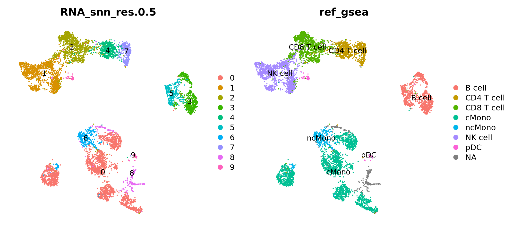
# Set the identity as louvain with resolution 0.5ctrl <-SetIdent(ctrl, value ="RNA_snn_res.0.5")ctrl <- ctrl %>%NormalizeData() %>%FindVariableFeatures() %>%ScaleData() %>%RunPCA(verbose = F) %>%RunUMAP(dims =1:30)
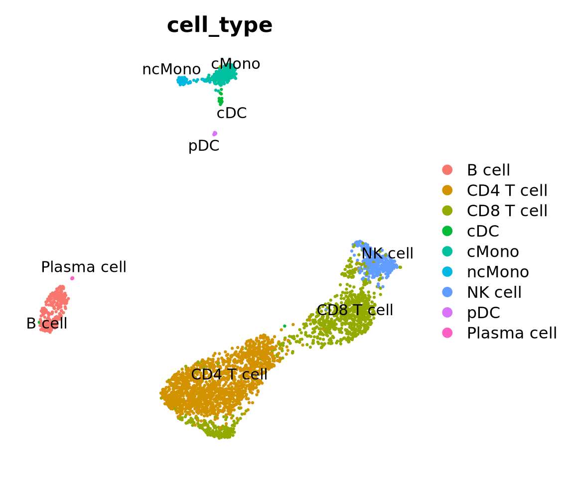
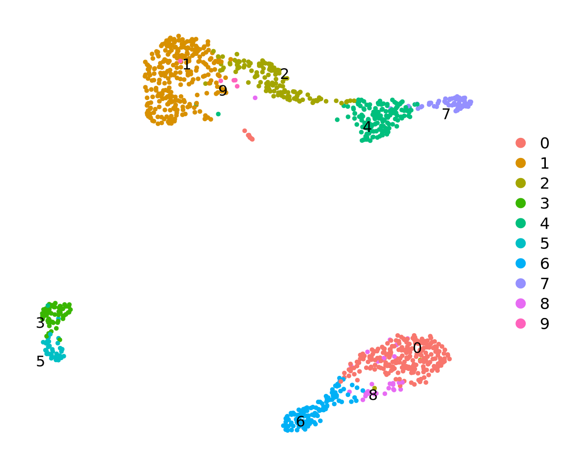
DimPlot(ctrl, label =TRUE, repel =TRUE) +NoAxes()
3 Label transfer
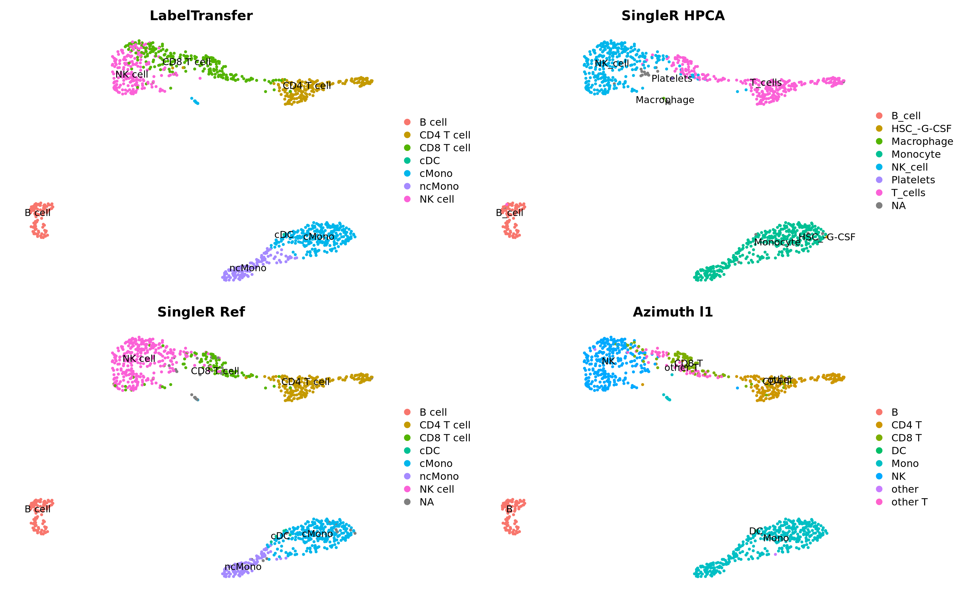
First we will run label transfer using a similar method as in the integration exercise. But, instead of CCA, which is the default for the FindTransferAnchors() function, we will use pcaproject, ie; the query dataset is projected onto the PCA of the reference dataset. Then, the labels of the reference data are predicted.
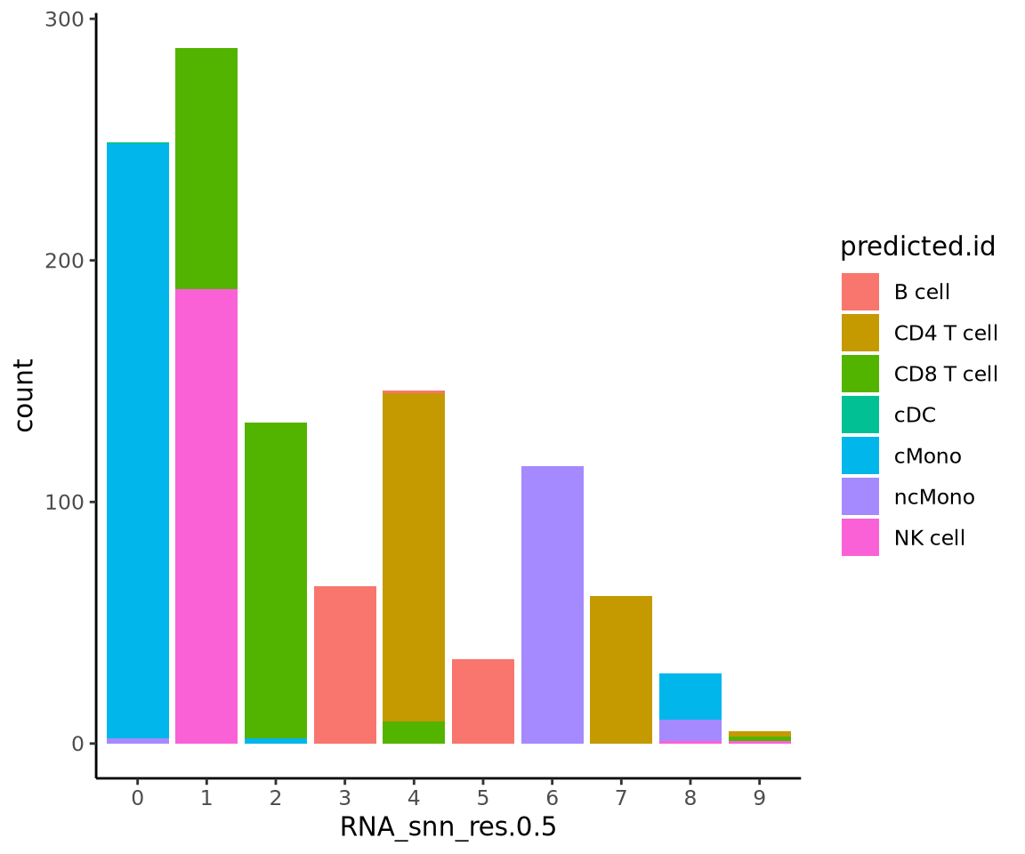
Now plot how many cells of each celltypes can be found in each cluster.
ggplot(ctrl@meta.data, aes(x = RNA_snn_res.0.5, fill = predicted.id)) +geom_bar() +theme_classic()
4 SinlgeR
SingleR is performs unbiased cell type recognition from single-cell RNA sequencing data, by leveraging reference transcriptomic datasets of pure cell types to infer the cell of origin of each single cell independently.
We first have to convert the Seurat object to a SingleCellExperiment object.
sce =as.SingleCellExperiment(ctrl)
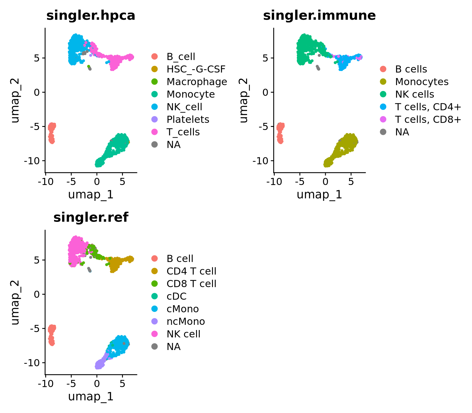
There are multiple datasets included in the celldex package that can be used for celltype prediction, here we will test two different ones, the DatabaseImmuneCellExpressionData and the HumanPrimaryCellAtlasData. In addition we will use the same reference dataset that we used for label transfer above but using SingleR instead.
DataFrame with 6 rows and 4 columns
                                                        scores        labels
                                                      <matrix>   <character>
ctrl_13_AGGTCATGTGCGAACA-13  0.06816733:0.0751051:0.186414:... T cells, CD4+
ctrl_13_CCTATCGGTCCCTCAT-13  0.00287888:0.0950319:0.386063:...      NK cells
ctrl_13_TCCTCCCTCGTTCATT-13  0.03637034:0.1055169:0.394461:...      NK cells
ctrl_13_CAACCAATCATCTATC-13  0.03449944:0.1335303:0.402336:...      NK cells
ctrl_13_TACGGTATCGGATTAC-13 -0.01303775:0.0707953:0.283801:...      NK cells
ctrl_13_AATAGAGAGTTCGGTT-13  0.08449581:0.1356925:0.273524:... T cells, CD4+
                            delta.next pruned.labels
                             <numeric>   <character>
ctrl_13_AGGTCATGTGCGAACA-13  0.1375513 T cells, CD4+
ctrl_13_CCTATCGGTCCCTCAT-13  0.1492478      NK cells
ctrl_13_TCCTCCCTCGTTCATT-13  0.1221984      NK cells
ctrl_13_CAACCAATCATCTATC-13  0.1514808      NK cells
ctrl_13_TACGGTATCGGATTAC-13  0.0617562      NK cells
ctrl_13_AATAGAGAGTTCGGTT-13  0.0660549 T cells, CD4+
There are multiple online resources with large curated datasets with methods to integrate and do label transfer. One such resource is Azimuth another one is Disco.
Here we will use the PBMC reference provided with Azimuth. Which in principle runs label transfer of your dataset onto a large curated reference. The first time you run the command, the pbmcref dataset will be downloaded to your local computer.
options(future.globals.maxSize =1e9)# will install the pbmcref dataset first time you run it.ctrl <-RunAzimuth(ctrl, reference ="pbmcref")
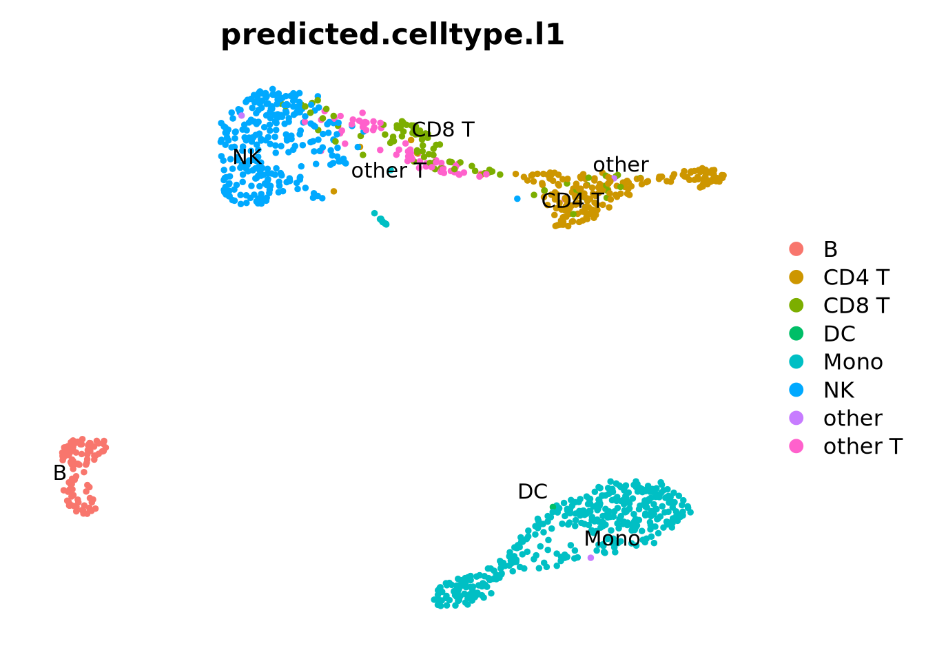
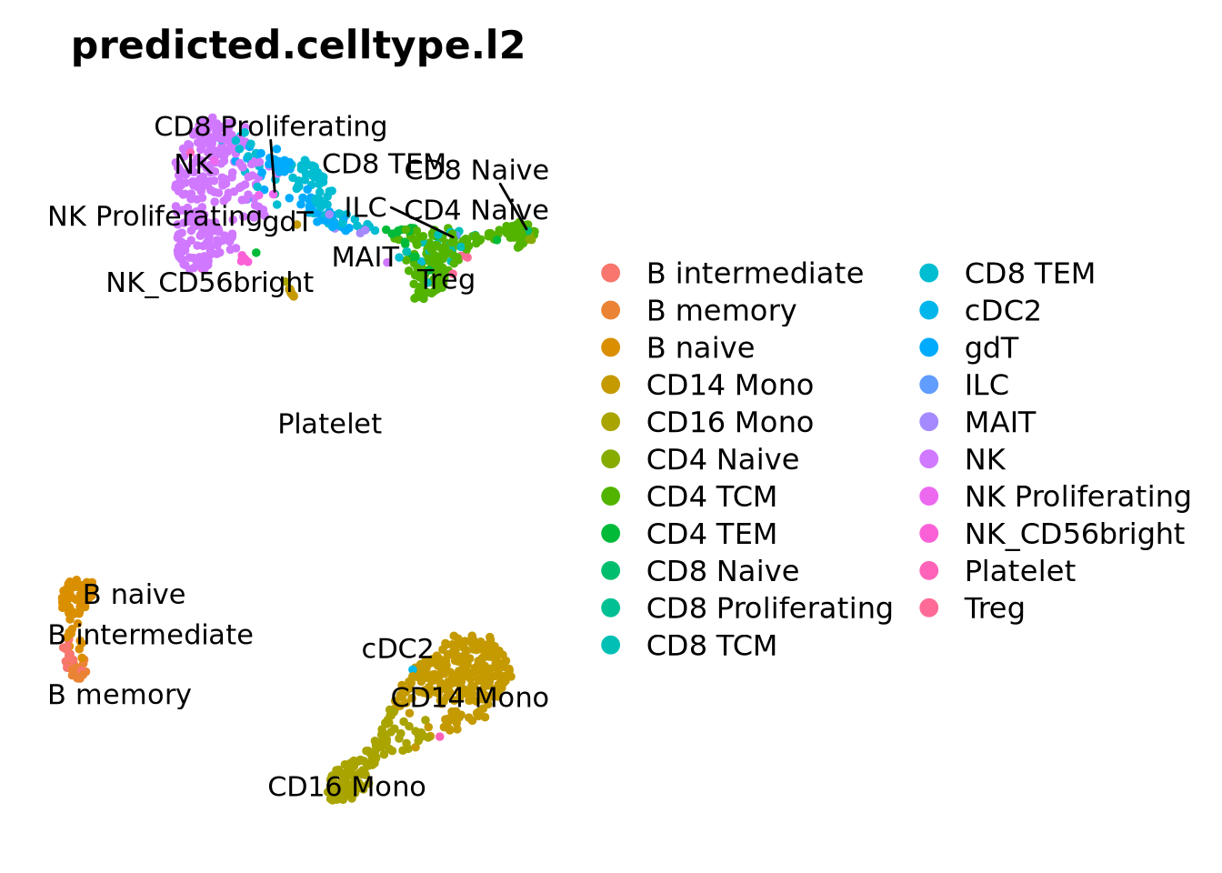
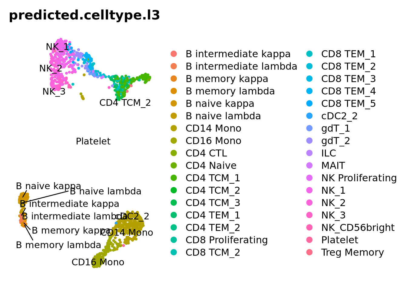
This dataset has predictions at 3 different levels of annotation wiht l1 being the more broad celltypes and l3 more detailed annotation.
Now we will compare the output of the two methods using the convenient function in scPred crossTab() that prints the overlap between two metadata slots.
crossTab(ctrl, "predicted.id", "singler.hpca")
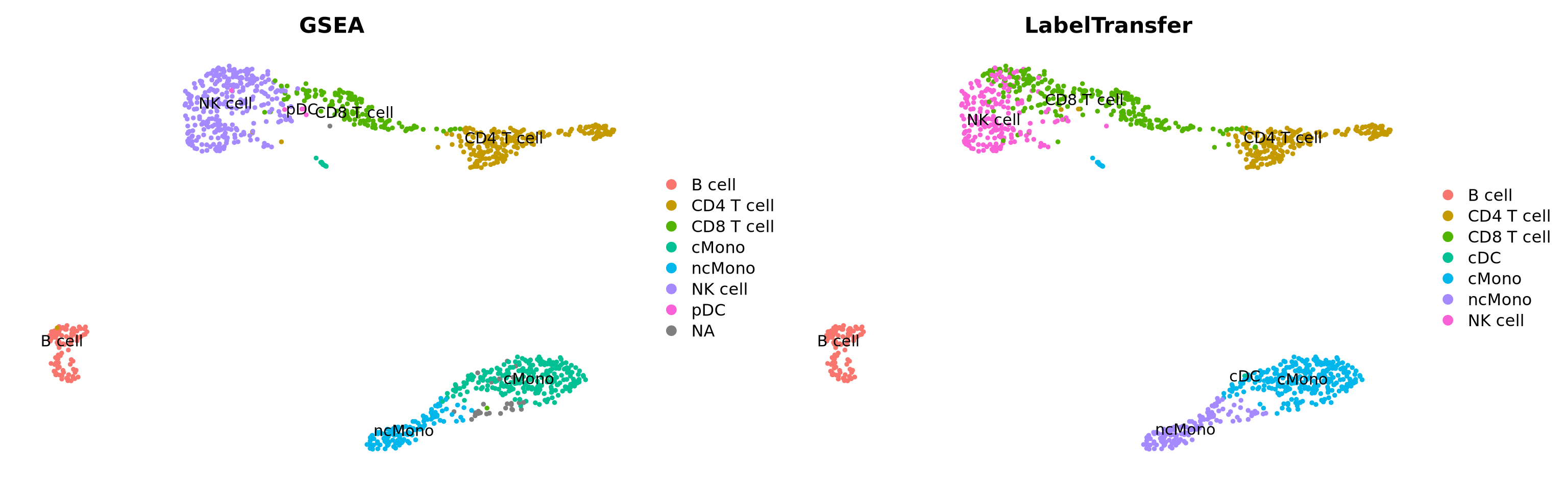
We can also plot all the different predictions side by side
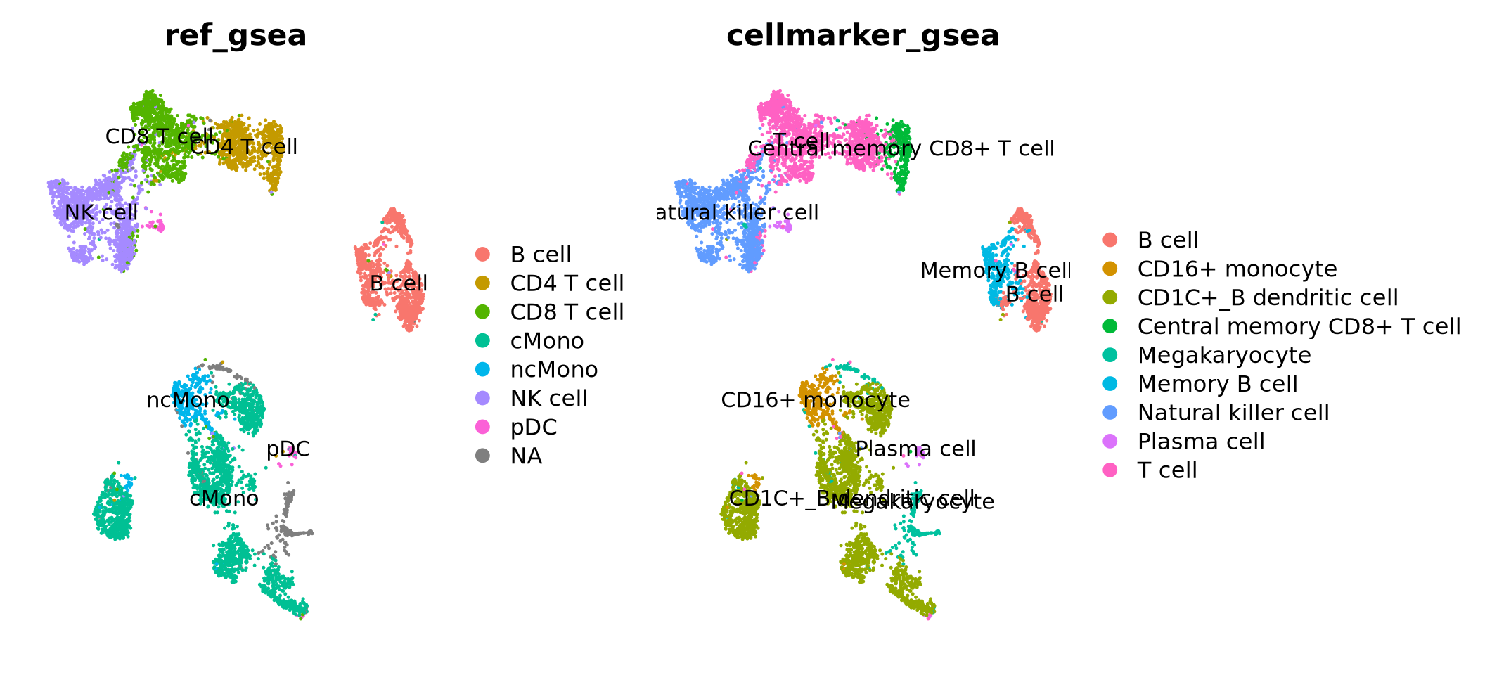
Another option, where celltype can be classified on cluster level is to use gene set enrichment among the DEGs with known markers for different celltypes. Similar to how we did functional enrichment for the DEGs in the differential expression exercise. There are some resources for celltype gene sets that can be used. Such as CellMarker, PanglaoDB or celltype gene sets at MSigDB. We can also look at overlap between DEGs in a reference dataset and the dataset you are analyzing.
7.1 DEG overlap
First, lets extract top DEGs for our Covid-19 dataset and the reference dataset. When we run differential expression for our dataset, we want to report as many genes as possible, hence we set the cutoffs quite lenient.
# run differential expression in our dataset, using clustering at resolution 0.5# first we need to join the layersalldata@active.assay ="RNA"alldata <-JoinLayers(object = alldata, layers =c("data","counts"))# set the clustering you want to use as the identity class.alldata <-SetIdent(alldata, value ="RNA_snn_res.0.5")DGE_table <-FindAllMarkers( alldata,logfc.threshold =0,test.use ="wilcox",min.pct =0.1,min.diff.pct =0,only.pos =TRUE,max.cells.per.ident =100,return.thresh =1,assay ="RNA")# split into a listDGE_list <-split(DGE_table, DGE_table$cluster)unlist(lapply(DGE_list, nrow))
# Compute differential gene expression in reference dataset (that has cell annotation)reference <-SetIdent(reference, value ="cell_type")reference_markers <-FindAllMarkers( reference,min.pct = .1,min.diff.pct = .2,only.pos = T,max.cells.per.ident =20,return.thresh =1)# Identify the top cell marker genes in reference dataset# select top 50 with hihgest foldchange among top 100 signifcant genes.reference_markers <- reference_markers[order(reference_markers$avg_log2FC, decreasing = T), ]reference_markers %>%group_by(cluster) %>%top_n(-100, p_val) %>%top_n(50, avg_log2FC) -> top50_cell_selection# Transform the markers into a listref_list <-split(top50_cell_selection$gene, top50_cell_selection$cluster)unlist(lapply(ref_list, length))
 CD8 T cell  CD4 T cell       cMono      B cell     NK cell         pDC
         30          15          50          50          50          50
     ncMono         cDC Plasma cell
         50          50          50
Now we can run GSEA for the DEGs from our dataset and check for enrichment of top DEGs in the reference dataset.
suppressPackageStartupMessages(library(fgsea))# run fgsea for each of the clusters in the listres <-lapply(DGE_list, function(x) { gene_rank <-setNames(x$avg_log2FC, x$gene) fgseaRes <-fgsea(pathways = ref_list, stats = gene_rank, nperm =10000)return(fgseaRes)})names(res) <-names(DGE_list)# You can filter and resort the table based on ES, NES or pvalueres <-lapply(res, function(x) { x[x$pval <0.1, ]})res <-lapply(res, function(x) { x[x$size >2, ]})res <-lapply(res, function(x) { x[order(x$NES, decreasing = T), ]})res
Selecting top significant overlap per cluster, we can now rename the clusters according to the predicted labels. OBS! Be aware that if you have some clusters that have non-significant p-values for all the gene sets, the cluster label will not be very reliable. Also, the gene sets you are using may not cover all the celltypes you have in your dataset and hence predictions may just be the most similar celltype. Also, some of the clusters have very similar p-values to multiple celltypes, for instance the ncMono and cMono celltypes are equally good for some clusters.
We have downloaded the celltype gene lists from http://bio-bigdata.hrbmu.edu.cn/CellMarker/CellMarker_download.html and converted the excel file to a csv for you. Read in the gene lists and do some filtering.
# Load the human marker tablemarkers <-read.delim("data/cell_marker_human.csv", sep =";")markers <- markers[markers$species =="Human", ]markers <- markers[markers$cancer_type =="Normal", ]# Filter by tissue (to reduce computational time and have tissue-specific classification)sort(unique(markers$tissue_type))
# run fgsea for each of the clusters in the listres <-lapply(DGE_list, function(x) { gene_rank <-setNames(x$avg_log2FC, x$gene) fgseaRes <-fgsea(pathways = celltype_list, stats = gene_rank, nperm =10000, scoreType ="pos")return(fgseaRes)})names(res) <-names(DGE_list)# You can filter and resort the table based on ES, NES or pvalueres <-lapply(res, function(x) { x[x$pval <0.01, ]})res <-lapply(res, function(x) { x[x$size >5, ]})res <-lapply(res, function(x) { x[order(x$NES, decreasing = T), ]})# show top 3 for each cluster.lapply(res, head, 3)
Do you think that the methods overlap well? Where do you see the most inconsistencies?
In this case we do not have any ground truth, and we cannot say which method performs best. You should keep in mind, that any celltype classification method is just a prediction, and you still need to use your common sense and knowledge of the biological system to judge if the results make sense.