Identify genes that are significantly over or under-expressed between conditions in specific cell populations.
Authors
Åsa Björklund
Paulo Czarnewski
Susanne Reinsbach
Roy Francis
Published
15-Apr-2026
Note
Code chunks run R commands unless otherwise specified.
In this tutorial we will cover differential gene expression, which comprises an extensive range of topics and methods. In single cell, differential expresison can have multiple functionalities such as identifying marker genes for cell populations, as well as identifying differentially regulated genes across conditions (healthy vs control). We will also cover controlling batch effect in your test.
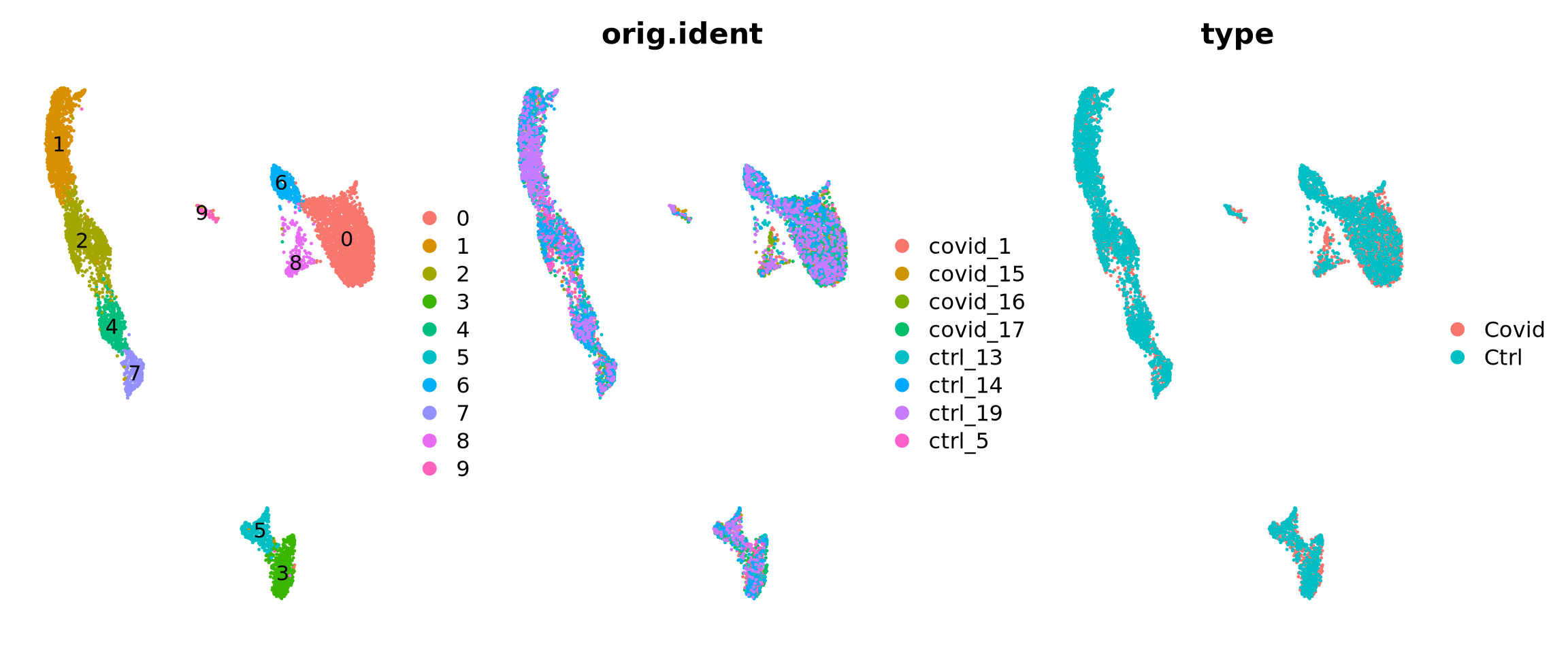
We can first load the data from the clustering session. Moreover, we can already decide which clustering resolution to use. First let’s define using the louvain clustering to identifying differentially expressed genes.
* checking for file ‘/tmp/RtmplTxCaT/remotes4b2fd277f8/immunogenomics-presto-7636b3d/DESCRIPTION’ ... OK
* preparing ‘presto’:
* checking DESCRIPTION meta-information ... OK
* cleaning src
* checking for LF line-endings in source and make files and shell scripts
* checking for empty or unneeded directories
* building ‘presto_1.0.0.tar.gz’
# download pre-computed data if missing or long computefetch_data <-TRUE# url for source and intermediate datapath_data <-"https://nextcloud.dc.scilifelab.se/public.php/webdav"curl_upass <-"-u zbC5fr2LbEZ9rSE:scRNAseq2025"path_file <-"data/covid/results/seurat_covid_qc_dr_int_cl.rds"if (!dir.exists(dirname(path_file))) dir.create(dirname(path_file), recursive =TRUE)if (fetch_data &&!file.exists(path_file)) download.file(url =file.path(path_data, "covid/results_seurat_2026/seurat_covid_qc_dr_int_cl.rds"), destfile = path_file, method ="curl", extra = curl_upass)alldata <-readRDS(path_file)
# Set the identity as louvain with resolution 0.5sel.clust <-"RNA_snn_res.0.5"alldata <-SetIdent(alldata, value = sel.clust)table(alldata@active.ident)
Let us first compute a ranking for the highly differential genes in each cluster. There are many different tests and parameters to be chosen that can be used to refine your results. When looking for marker genes, we want genes that are positively expressed in a cell type and possibly not expressed in others.
For differential expression it is important to use the RNA assay, for most tests we will use the logtransformed counts in the data slot. With Seurat v5 the data may be split into layers depending on what you did with the data beforehand. So first, lets check what we have in our object:
Now we can run the function FindAllMarkers that will run each of the clusters vs the rest. As you can see, there are some filtering criteria to remove genes that do not have certain log2FC or percent expressed. Here we only test for upregulated genes, so the only.pos parameter is set to TRUE.
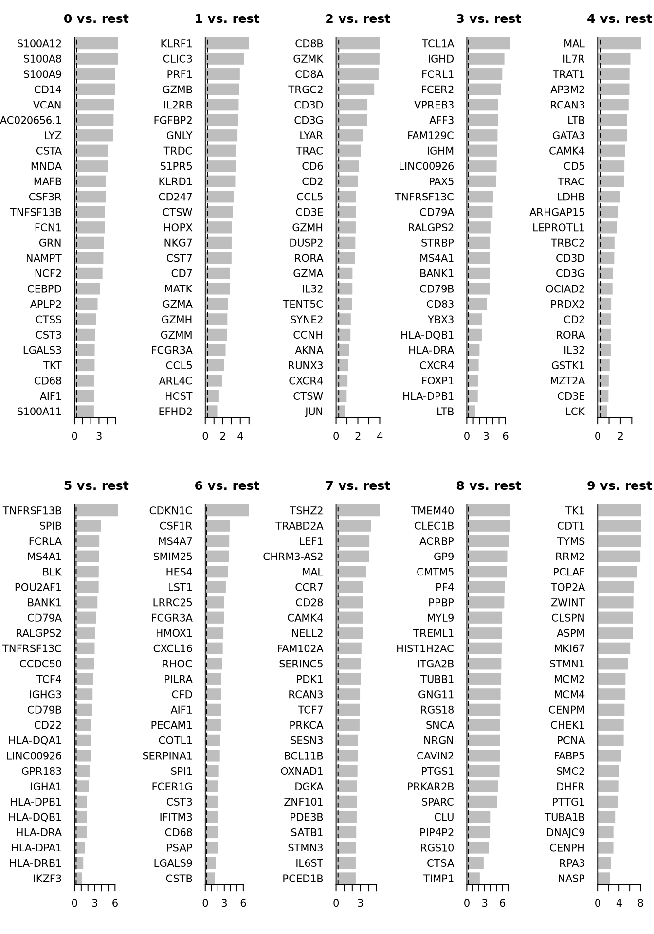
We can now select the top 25 overexpressed genes for plotting.
markers_genes %>%group_by(cluster) %>%top_n(-25, p_val_adj) %>%# In case of tied p-values, further select the top 25 genes by fold-changetop_n(25, avg_log2FC) -> top25head(top25)
par(mfrow =c(2, 5), mar =c(4, 6, 3, 1))for (i inunique(top25$cluster)) {barplot(sort(setNames(top25$avg_log2FC, top25$gene)[top25$cluster == i], F),horiz = T, las =1, main =paste0(i, " vs. rest"), border ="white", yaxs ="i" )abline(v =c(0, 0.25), lty =c(1, 2))}
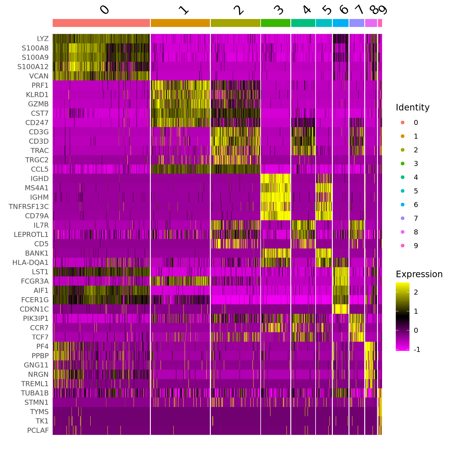
We can visualize them as a heatmap. Here we are selecting the top 5.
markers_genes %>%group_by(cluster) %>%slice_min(p_val_adj, n =5, with_ties =FALSE) -> top5# create a scale.data slot for the selected genesalldata <-ScaleData(alldata, features =as.character(unique(top5$gene)), assay ="RNA")DoHeatmap(alldata, features =as.character(unique(top5$gene)), group.by = sel.clust, assay ="RNA")
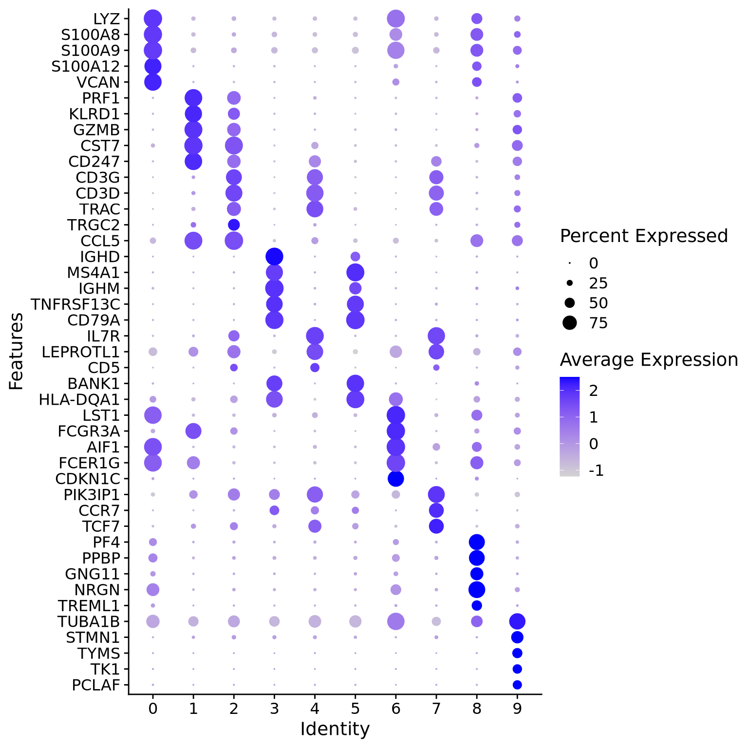
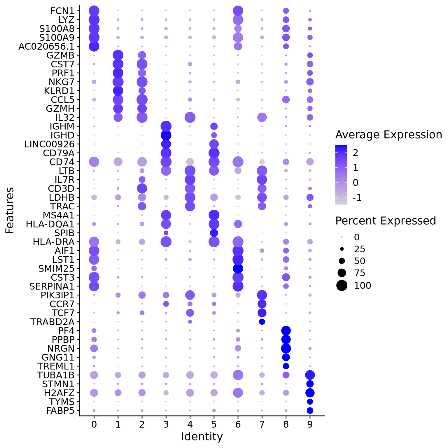
Another way is by representing the overall group expression and detection rates in a dot-plot.
DotPlot(alldata, features =rev(as.character(unique(top5$gene))), group.by = sel.clust, assay ="RNA") +coord_flip()
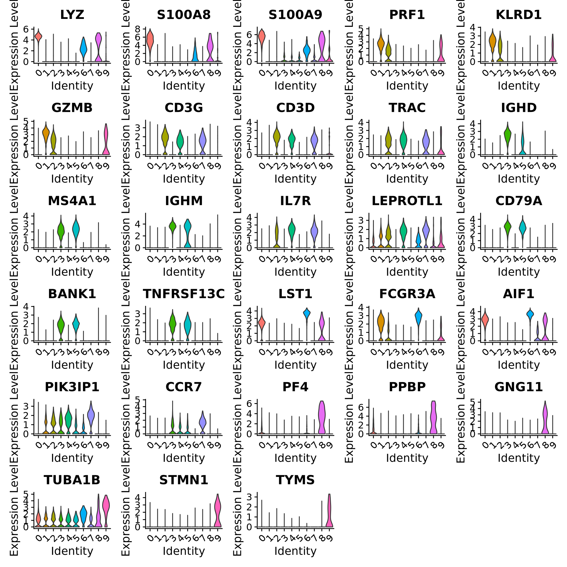
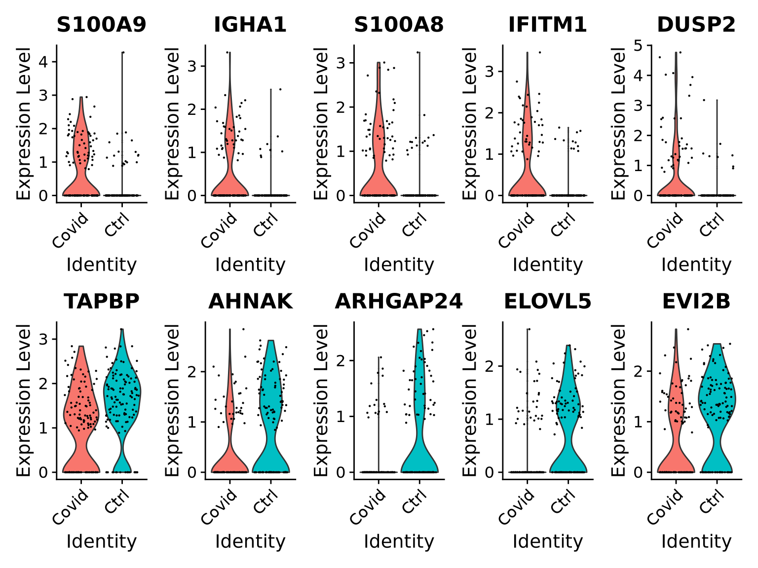
We can also plot a violin plot for each gene.
# take top 3 genes per cluster/top5 %>%group_by(cluster) %>%top_n(-3, p_val) -> top3# set pt.size to zero if you do not want all the points to hide the violin shapes, or to a small value like 0.1VlnPlot(alldata, features =as.character(unique(top3$gene)), ncol =5, group.by = sel.clust, assay ="RNA", pt.size =0)
Discuss
Take a screenshot of those results and re-run the same code above with another test: “wilcox” (Wilcoxon Rank Sum test), “bimod” (Likelihood-ratio test), “roc” (Identifies ‘markers’ of gene expression using ROC analysis),“t” (Student’s t-test),“negbinom” (negative binomial generalized linear model),“poisson” (poisson generalized linear model), “LR” (logistic regression), “MAST” (hurdle model), “DESeq2” (negative binomial distribution).
1.1 DGE with equal amount of cells
The number of cells per cluster differ quite a bit in this data
Hence when we run FindAllMarkers one cluster vs rest, the largest cluster (cluster 0) will dominate the “rest” and influence the results the most. So it is often a good idea to subsample the clusters to an equal number of cells before running differential expression for one vs rest. We can select a fixed number of cells per cluster with the function WhichCells and the argument downsample.
sub <-subset(alldata, cells =WhichCells(alldata, downsample =300))table(sub@active.ident)
markers_genes_sub %>%group_by(cluster) %>%slice_min(p_val_adj, n =5, with_ties =FALSE) -> top5_subDotPlot(alldata, features =rev(as.character(unique(top5_sub$gene))), group.by = sel.clust, assay ="RNA") +coord_flip()
2 DGE across conditions
The second way of computing differential expression is to answer which genes are differentially expressed within a cluster. For example, in our case we have libraries comming from patients and controls and we would like to know which genes are influenced the most in a particular cell type. For this end, we will first subset our data for the desired cell cluster, then change the cell identities to the variable of comparison (which now in our case is the type, e.g. Covid/Ctrl).
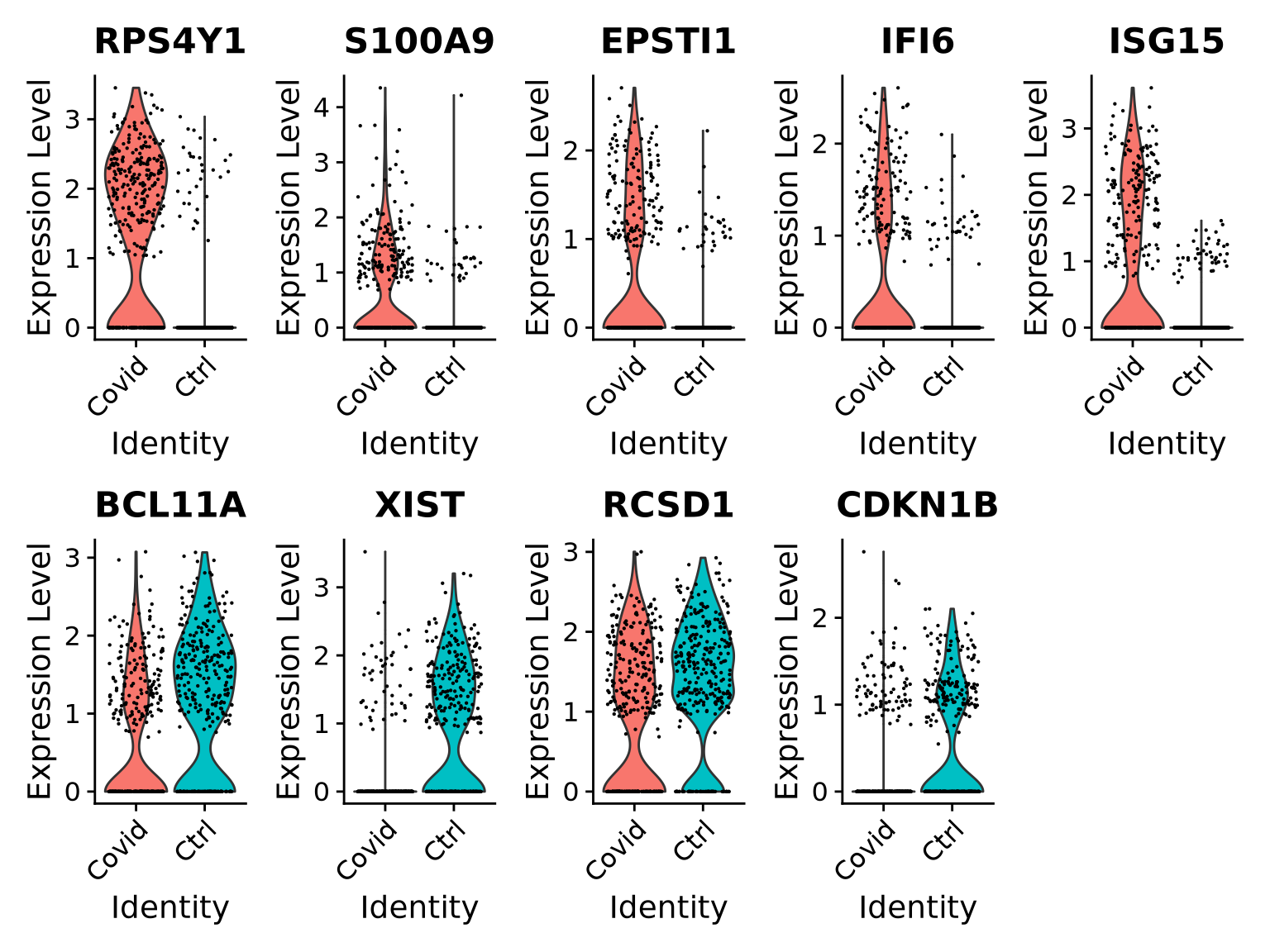
# select all cells in cluster 3cell_selection <-subset(alldata, cells =colnames(alldata)[alldata@meta.data[, sel.clust] ==3])cell_selection <-SetIdent(cell_selection, value ="type")# Compute differentiall expressionDGE_cell_selection <-FindAllMarkers(cell_selection,logfc.threshold =0.2,test.use ="wilcox",min.pct =0.1,min.diff.pct =0.2,only.pos =TRUE,max.cells.per.ident =50,assay ="RNA")
As you can see, we have many sex chromosome related genes among the top DE genes. And if you remember from the QC lab, we have unbalanced sex distribution among our subjects, so this may not be related to covid at all.
2.1 Remove sex chromosome genes
To remove some of the bias due to unbalanced sex in the subjects, we can remove the sex chromosome related genes.
gene.info <-read.csv(genes_file) # was created in the QC exerciseauto.genes <- gene.info$external_gene_name[!(gene.info$chromosome_name %in%c("X", "Y"))]cell_selection@active.assay <-"RNA"keep.genes <-intersect(rownames(cell_selection), auto.genes)cell_selection <- cell_selection[keep.genes, ]# then renormalize the datacell_selection <-NormalizeData(cell_selection)
Rerun differential expression:
# Compute differential expressionDGE_cell_selection <-FindMarkers(cell_selection,ident.1 ="Covid", ident.2 ="Ctrl",logfc.threshold =0.2, test.use ="wilcox", min.pct =0.1,min.diff.pct =0.2, assay ="RNA")# Define as Covid or Ctrl in the df and add a gene columnDGE_cell_selection$direction <-ifelse(DGE_cell_selection$avg_log2FC >0, "Covid", "Ctrl")DGE_cell_selection$gene <-rownames(DGE_cell_selection)DGE_cell_selection %>%group_by(direction) %>%top_n(-5, p_val) %>%arrange(direction) -> top5_cell_selection
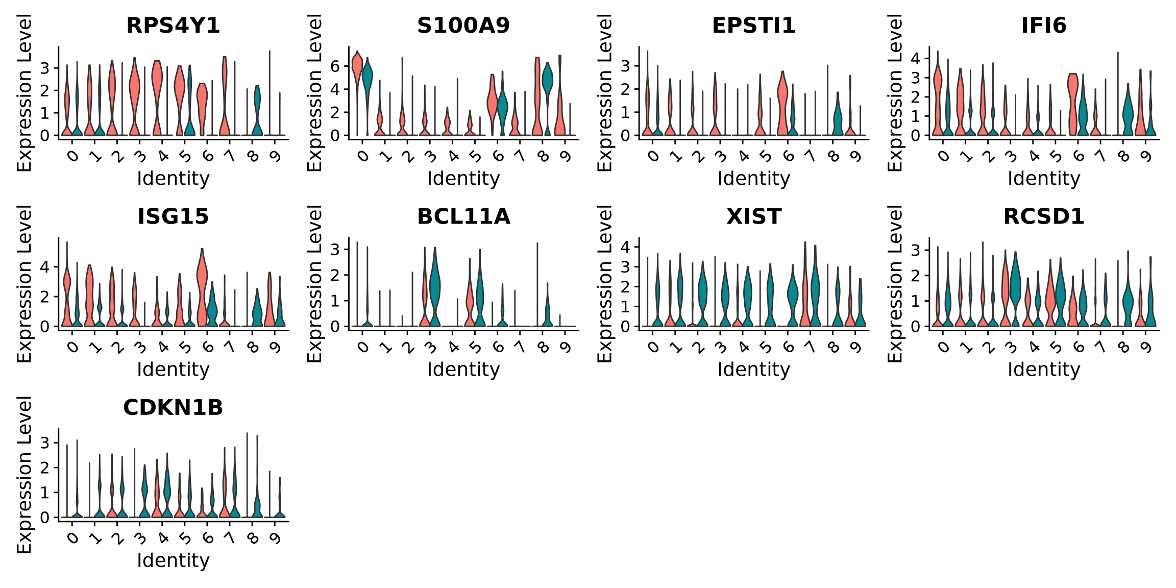
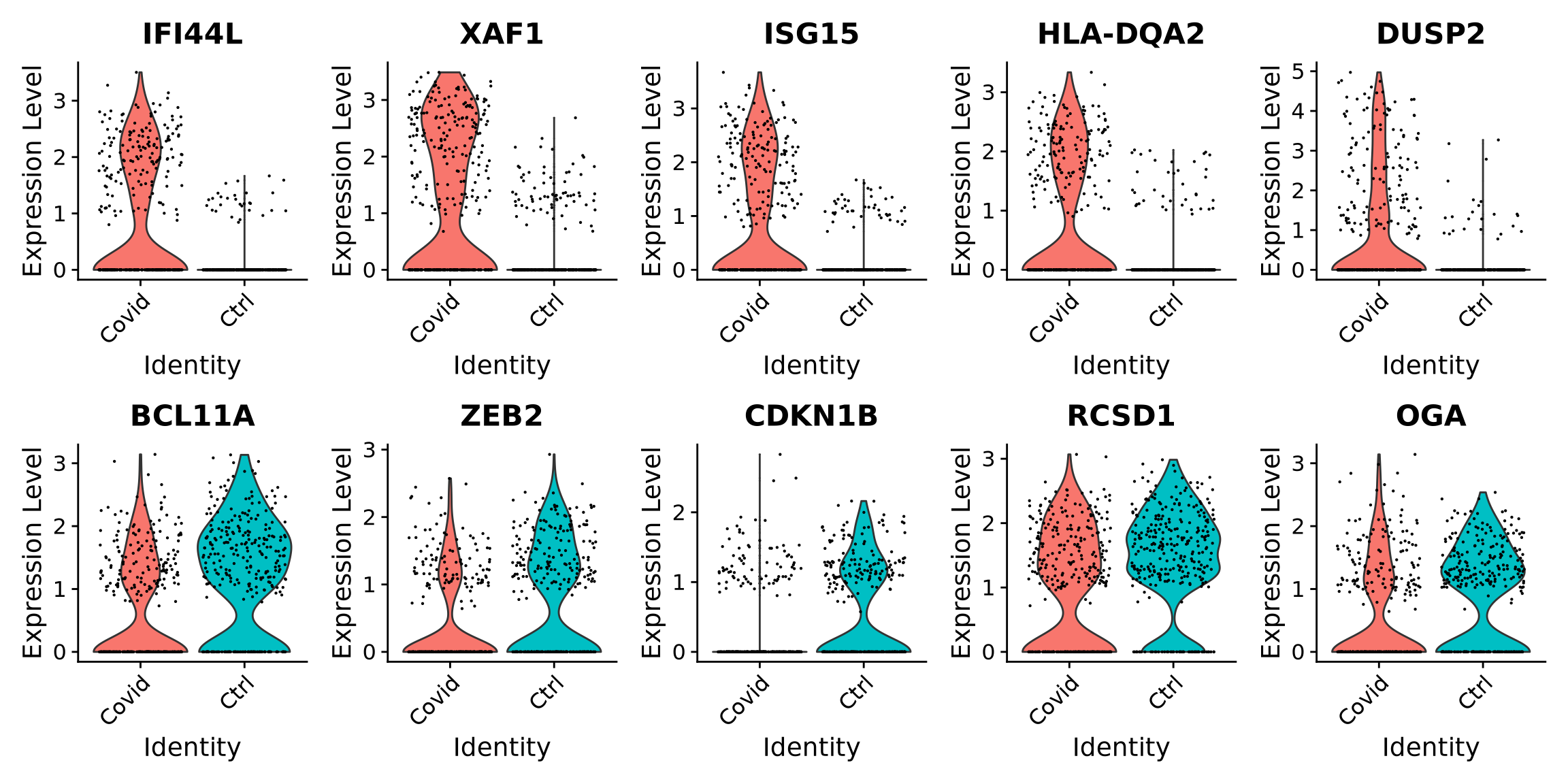
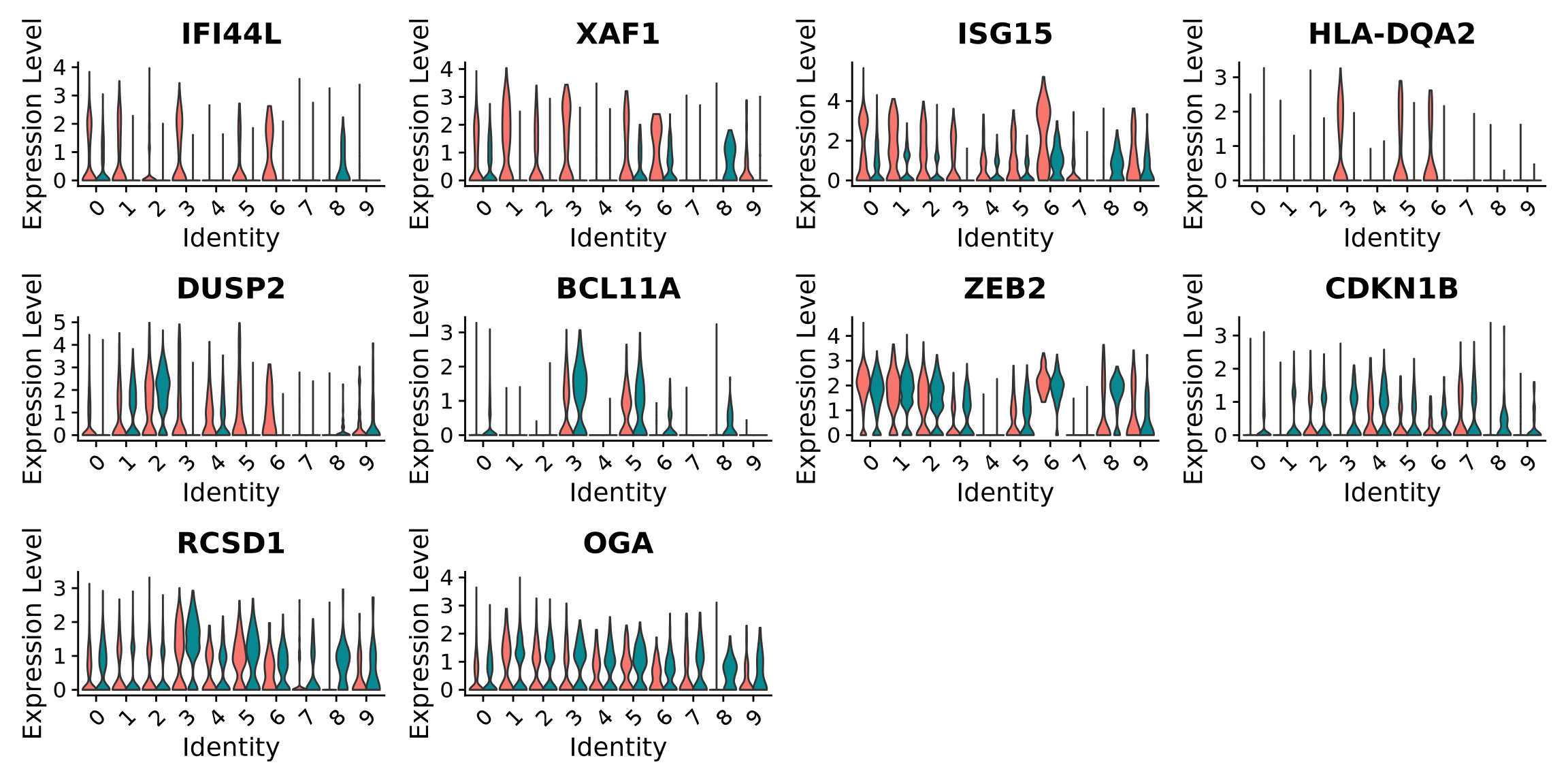
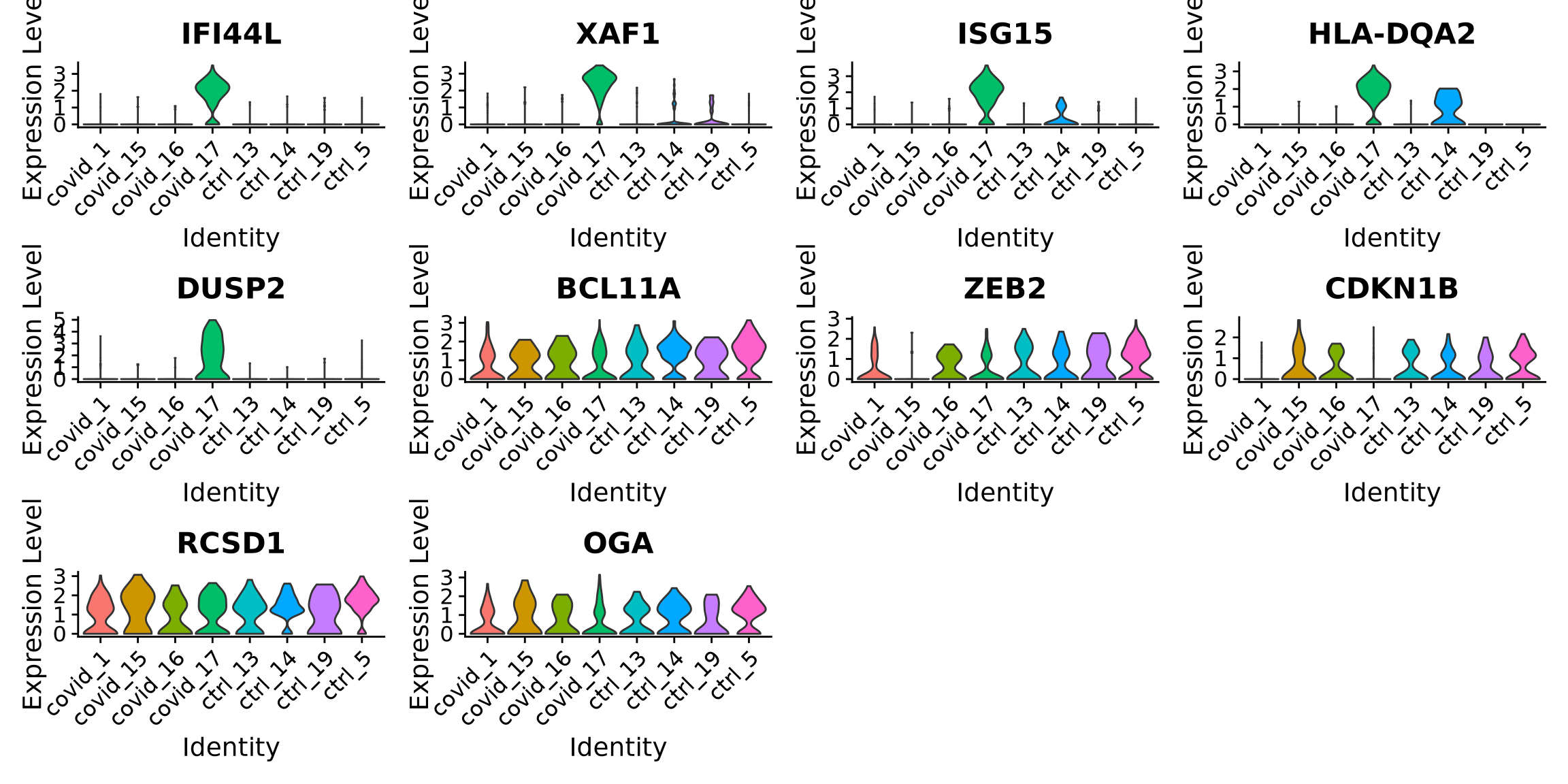
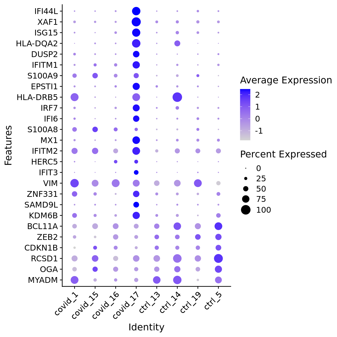
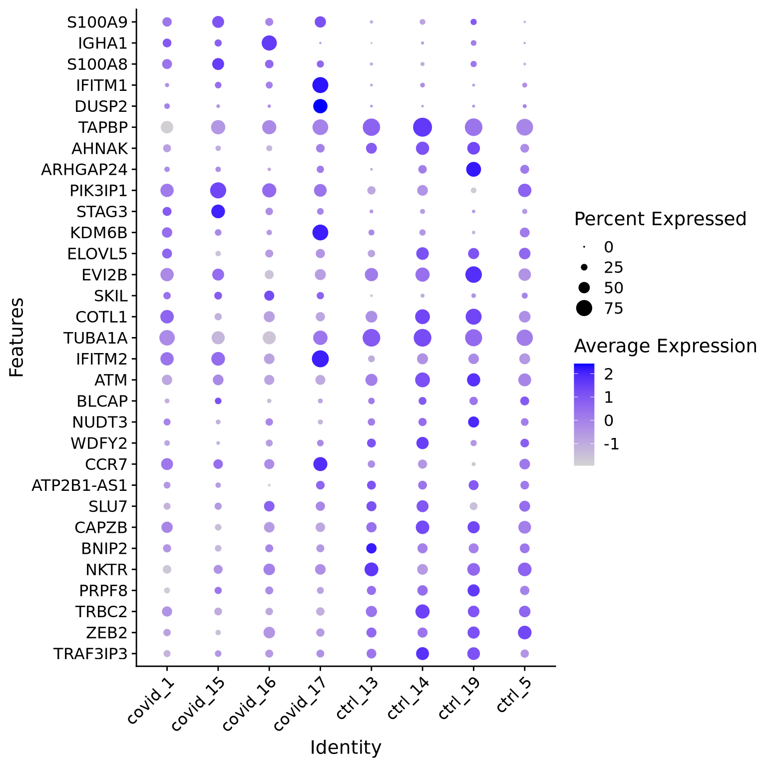
When we are testing for Covid vs Control, we are running a DGE test for 4 vs 4 individuals. That will be very sensitive to sample differences unless we find a way to control for it. So first, let’s check how the top DEGs are expressed across the individuals within cluster 3:
It looks much better now. But if we look per patient you can see that we still have some genes that are dominated by a single patient.
Why do you think this is?
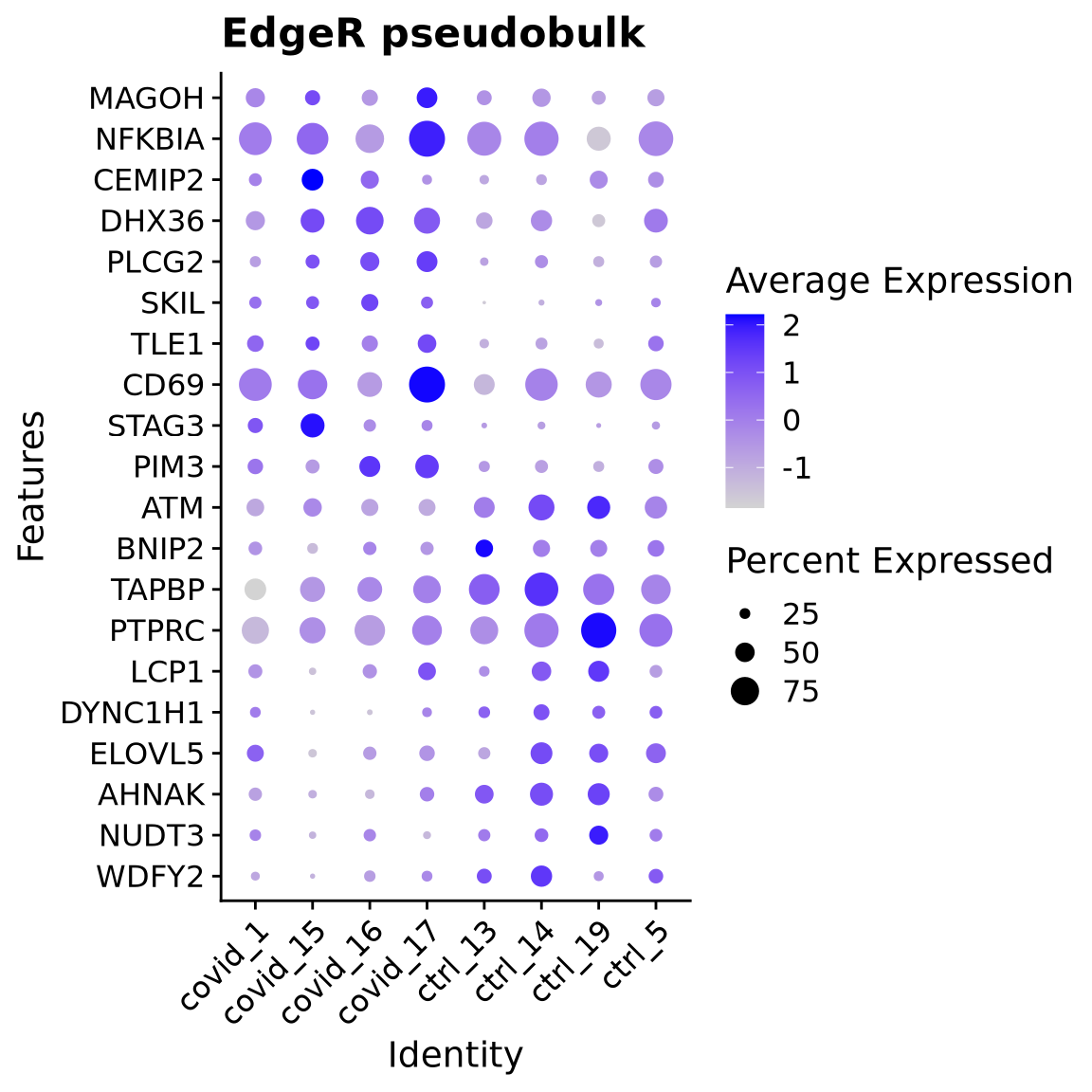
5 Pseudobulk
One option is to treat the samples as pseudobulks and do differential expression for the 4 patients vs 4 controls. You do lose some information about cell variability within each patient, but instead you gain the advantage of mainly looking for effects that are seen in multiple patients.
However, having only 4 patients is perhaps too low, with many more patients it will work better to run pseudobulk analysis.
For a fair comparison we should have equal number of cells per sample when we create the pseudobulk with AggregateExpression. For pseudobulk it is recommended to use the subsampled object so that you have similar amount of cells into each pseudobulk calculation. A biased number of cells will strongly influence the differential expression you run with the pseudobulk.
As you can see, even if we find few genes, they seem to make sense across all the patients.
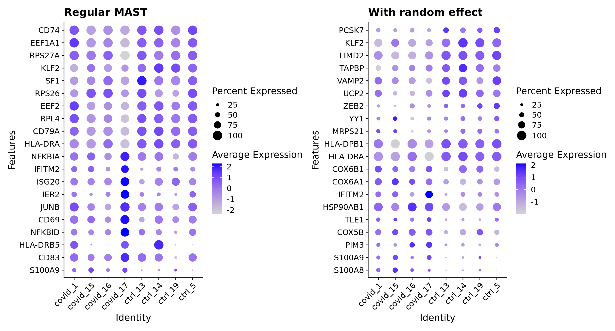
6 MAST random effect
MAST has the option to add a random effect for the patient when running DGE analysis. It is quite slow, even with this small dataset, so it may not be practical for a larger dataset unless you have access to a compute cluster.
We will run MAST with and without patient info as random effect and compare the results
First, filter genes in part to speed up the process but also to avoid too many warnings in the model fitting step of MAST. We will keep genes that are expressed with at least 2 reads in 2 covid patients or 2 controls.
# select genes that are expressed in at least 2 patients or 2 ctrls with > 2 reads.nPatient <-sapply(unique(cell_selection$orig.ident), function(x) {rowSums(cell_selection@assays$RNA@layers$counts[, cell_selection$orig.ident == x] >2)})nCovid <-rowSums(nPatient[, 1:4] >2)nCtrl <-rowSums(nPatient[, 5:8] >2)sel <- nCovid >=2| nCtrl >=2cell_selection_sub <- cell_selection[sel, ]
Set up the MAST object.
# create the feature datafData <-data.frame(primerid =rownames(cell_selection_sub))m <- cell_selection_sub@meta.datam$wellKey <-rownames(m)# make sure type and orig.ident are factorsm$orig.ident <-factor(m$orig.ident)m$type <-factor(m$type)sca <- MAST::FromMatrix(exprsArray =as.matrix(x = cell_selection_sub@assays$RNA@layers$data),check_sanity =FALSE, cData = m, fData = fData)
First, run the regular MAST analysis without random effects
# takes a while to run, so save a file to tmpdir in case you have to rerun the codetmpdir <-"data/covid/results/tmp_dge"dir.create(tmpdir, showWarnings = F)tmpfile1 <-file.path(tmpdir, "mast_bayesglm_cl4.Rds")if (file.exists(tmpfile1)) { fcHurdle1 <-readRDS(tmpfile1)} else { zlmCond <-suppressMessages(MAST::zlm(~ type + nFeature_RNA, sca, method ="bayesglm", ebayes = T)) summaryCond <-suppressMessages(MAST::summary(zlmCond, doLRT ="typeCtrl")) summaryDt <- summaryCond$datatable fcHurdle <-merge(summaryDt[summaryDt$contrast =="typeCtrl"& summaryDt$component =="logFC", c(1, 7, 5, 6, 8)], summaryDt[summaryDt$contrast =="typeCtrl"& summaryDt$component =="H", c(1, 4)], by ="primerid") fcHurdle1 <- stats::na.omit(as.data.frame(fcHurdle))saveRDS(fcHurdle1, tmpfile1)}
As you can see, we have lower significance for the genes with the random effect added.
Dotplot for top 10 genes in each direction:
p1 <-DotPlot(cell_selection, features = mastN, group.by ="orig.ident", assay ="RNA") +coord_flip() +RotatedAxis() +ggtitle("Regular MAST")p2 <-DotPlot(cell_selection, features = mastR, group.by ="orig.ident", assay ="RNA") +coord_flip() +RotatedAxis() +ggtitle("With random effect")p1 + p2
Discuss
You have now run DGE analysis for Covid vs Ctrl in cluster 3 with several diffent methods. Have a look at the different results. Where did you get more/less significant genes? Which results would you like to present in a paper? Discuss with a neighbor which one you think looks best and why.
7 Gene Set Analysis (GSA)
7.1 Hypergeometric enrichment test
Having a defined list of differentially expressed genes, you can now look for their combined function using hypergeometric test.
In this case we will use the DGE from MAST with random effect to run enrichment analysis.
# Load additional packageslibrary(enrichR)# Check available databases to perform enrichment (then choose one)enrichR::listEnrichrDbs()
Uploading data to Enrichr... Done.
  Querying GO_Biological_Process_2025... Done.
Parsing results... Done.
Some databases of interest: GO_Biological_Process_2017bKEGG_2019_HumanKEGG_2019_MouseWikiPathways_2019_HumanWikiPathways_2019_Mouse
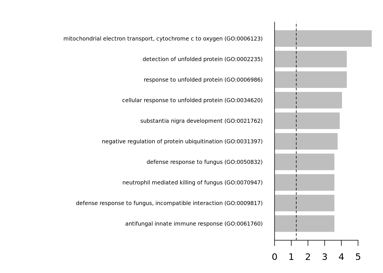
You visualize your results using a simple barplot, for example:
Besides the enrichment using hypergeometric test, we can also perform gene set enrichment analysis (GSEA), which scores ranked genes list (usually based on fold changes) and computes permutation test to check if a particular gene set is more present in the Up-regulated genes, among the DOWN_regulated genes or not differentially regulated.
Before, we ran FindMarkers() with the default settings for reporting only significantly up/down regulated genes, but now we need statistics on a larger set of genes, so we will have to rerun the test with more lenient cutoffs. We will not use it now but this is how it should be run:
## OBS! No need to runsub_data <-SetIdent(sub_data, value ="type")DGE_cell_selection2 <-FindMarkers( sub_data,ident.1 ="Covid",logfc.threshold =-Inf,test.use ="wilcox",min.pct =0.05,min.diff.pct =0,only.pos =FALSE,max.cells.per.ident =50,assay ="RNA")# Create a gene rank based on the gene expression fold changegene_rank <-setNames(DGE_cell_selection2$avg_log2FC, casefold(rownames(DGE_cell_selection2), upper = T))
In this case we will use the results from MAST with random effect to run GSEA, and we will use the Z-score from MAST to sort the genes.
gene_rank <-setNames(fcHurdle2$z, casefold(fcHurdle2$primerid, upper = T))# set infinite values to 100.inf =is.infinite(gene_rank)gene_rank[inf] =100*sign(gene_rank[inf])
Once our list of genes are sorted, we can proceed with the enrichment itself. We can use the package to get gene set from the Molecular Signature Database (MSigDB) and select KEGG pathways as an example.
library(msigdbr)# Download gene setsmsigdbgmt <- msigdbr::msigdbr("Homo sapiens")msigdbgmt <-as.data.frame(msigdbgmt)# List available gene setsunique(msigdbgmt$gs_subcat)
# Subset which gene set you want to use.msigdbgmt_subset <- msigdbgmt[msigdbgmt$gs_subcat =="CP:WIKIPATHWAYS", ]gmt <-lapply(unique(msigdbgmt_subset$gs_name), function(x) { msigdbgmt_subset[msigdbgmt_subset$gs_name == x, "gene_symbol"]})names(gmt) <-unique(paste0(msigdbgmt_subset$gs_name, "_", msigdbgmt_subset$gs_exact_source))
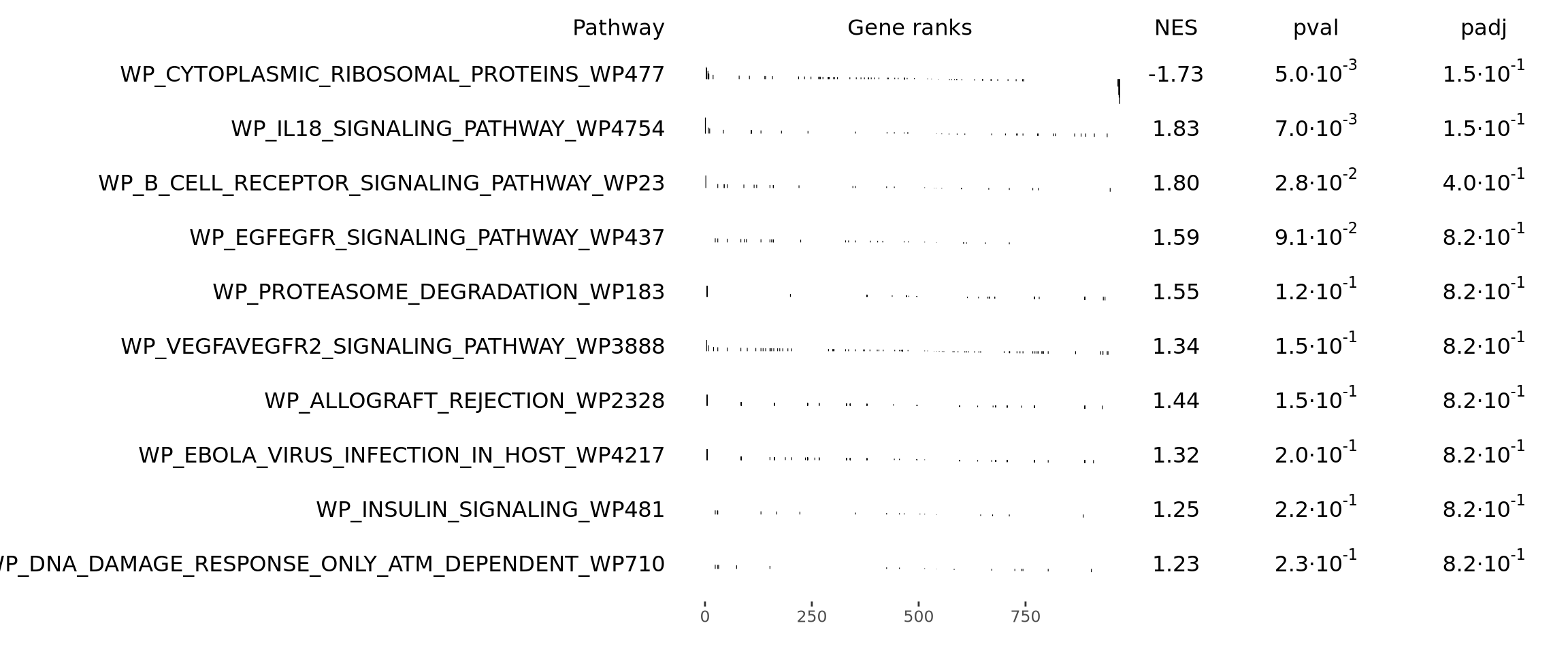
Next, we will run GSEA. This will result in a table containing information for several pathways. We can then sort and filter those pathways to visualize only the top ones. You can select/filter them by either p-value or normalized enrichment score (NES).
library(fgsea)# Perform enrichemnt analysisfgseaRes <-fgsea(pathways = gmt, stats = gene_rank, minSize =15, maxSize =500)fgseaRes <- fgseaRes[order(fgseaRes$pval, decreasing = F), ]# Filter the results table to show only the top 10 UP or DOWN regulated processes (optional)top10_UP <- fgseaRes$pathway[1:10]# Nice summary table (shown as a plot)plotGseaTable(gmt[top10_UP], gene_rank, fgseaRes, gseaParam =0.5)
Discuss
Which KEGG pathways are upregulated in this cluster? Which KEGG pathways are dowregulated in this cluster? Change the pathway source to another gene set (e.g. CP:WIKIPATHWAYS or CP:REACTOME or CP:BIOCARTA or GO:BP) and check the if you get similar results?