suppressPackageStartupMessages({
    library(Seurat)
    library(ggplot2)
    library(patchwork)
    library(basilisk)
})

condapath = "/usr/local/conda/envs/seurat"
Note
Code chunks run R commands unless otherwise specified.
In this tutorial we will look at different ways of integrating multiple single cell RNA-seq datasets. We will explore a few different methods to correct for batch effects across datasets. Seurat uses the data integration method presented in Comprehensive Integration of Single Cell Data, while Scran and Scanpy use a mutual Nearest neighbour method (MNN). Below you can find a list of some methods for single data integration:
| Markdown | Language | Library | Ref |
|---|---|---|---|
| CCA | R | Seurat | Cell |
| MNN | R/Python | Scater/Scanpy | Nat. Biotech. |
| Conos | R | conos | Nat. Methods |
| Harmony | R | Harmony | Nat. Methods |
| Scanorama | Python | scanorama | Nat. Biotech. |
1 Data preparation
Let’s first load necessary libraries and the data saved in the previous lab.
# download pre-computed data if missing or long compute
fetch_data <- TRUE

# url for source and intermediate data
path_data <- "https://nextcloud.dc.scilifelab.se/public.php/webdav"
curl_upass <- "-u zbC5fr2LbEZ9rSE:scRNAseq2025"

path_file <- "data/covid/results/seurat_covid_qc_dr.rds"
if (!dir.exists(dirname(path_file))) dir.create(dirname(path_file), recursive = TRUE)
if (fetch_data && !file.exists(path_file)) download.file(url = file.path(path_data, "covid/results_seurat_2026/seurat_covid_qc_dr.rds"), destfile = path_file, method = "curl", extra = curl_upass)

alldata <- readRDS(path_file)
print(names(alldata@reductions))
[1] "pca" "umap" "tsne"
[4] "UMAP10_on_PCA" "UMAP_on_ScaleData"With Seurat5 we can split the RNA assay into multiple Layers with one count matrix and one data matrix per sample. When we then run FindVariableFeatures on the object it will run it for each of the samples separately, but also compute the overall variable features by combining their ranks.
# get the variable genes from all the datasets without batch information.
hvgs_old = VariableFeatures(alldata)

# now split the object into layers
alldata[["RNA"]] <- split(alldata[["RNA"]], f = alldata$orig.ident)

# detect HVGs
alldata <- FindVariableFeatures(alldata, selection.method = "vst", nfeatures = 2000, verbose = FALSE)

# to get the HVGs for each layer we have to fetch them individually
data.layers <- Layers(alldata)[grep("data.",Layers(alldata))]
print(data.layers)
[1] "data.ctrl_13" "data.ctrl_14" "data.ctrl_19" "data.ctrl_5"
[5] "data.covid_15" "data.covid_16" "data.covid_17" "data.covid_1" hvgs_per_dataset <- lapply(data.layers, function(x) VariableFeatures(alldata, layer = x) )
names(hvgs_per_dataset) = data.layers
# also add in the variable genes that was selected on the whole dataset and the old ones
hvgs_per_dataset$all <- VariableFeatures(alldata)
hvgs_per_dataset$old <- hvgs_old
temp <- unique(unlist(hvgs_per_dataset))
overlap <- sapply( hvgs_per_dataset , function(x) { temp %in% x } )
pheatmap::pheatmap(t(overlap*1),cluster_rows = F ,
color = c("grey90","grey20"))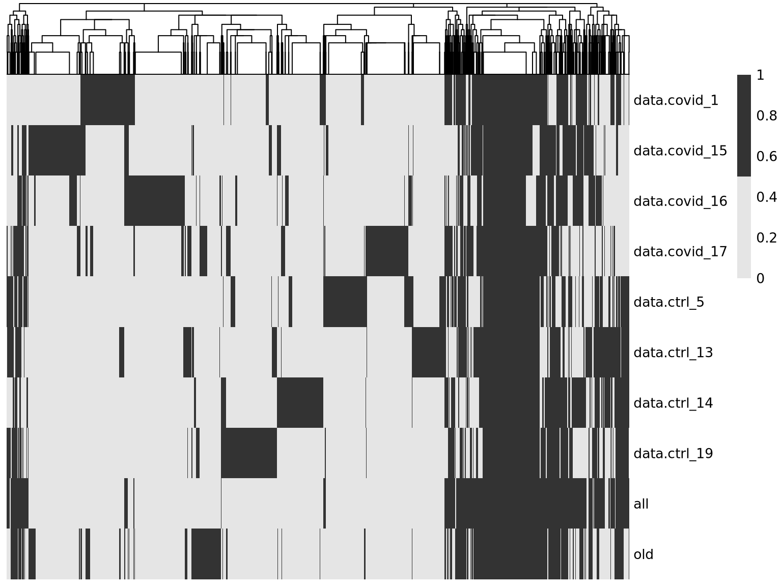
As you can see, there are a lot of genes that are variable in just one dataset. There are also some genes in the gene set that was selected using all the data that are not variable in any of the individual datasets. These are most likely genes driven by batch effects.
A better way to select features for integration is to combine the information on variable genes across the dataset. This is what we have in the all section where the ranks of the variable features in the different datasets is combined.
Discuss
Did you understand the difference between running variable gene selection per dataset and combining them vs running it on all samples together. Can you think of any situation where it would be best to run it on all samples and a situation where it should be done by batch?
For all downstream integration we will use this set of genes so that it is comparable across the methods. Before doing anything else we need to rerun ScaleData and PCA with that set of genes.
hvgs_all = hvgs_per_dataset$all

alldata = ScaleData(alldata, features = hvgs_all, vars.to.regress = c("percent_mito", "nFeature_RNA"))
alldata = RunPCA(alldata, features = hvgs_all, verbose = FALSE)
2 CCA
In Seurat v4 we run the integration in two steps, first finding anchors between datasets with FindIntegrationAnchors() and then running the actual integration with IntegrateData(). Since Seurat v5 this is done in a single command using the function IntegrateLayers(), we specify the name for the integration as integrated_cca.
alldata <- IntegrateLayers(object = alldata,
                           method = CCAIntegration, orig.reduction = "pca",
                           new.reduction = "integrated_cca", verbose = FALSE)
We should now have a new dimensionality reduction slot (integrated_cca) in the object:
names(alldata@reductions)[1] "pca" "umap" "tsne"
[4] "UMAP10_on_PCA" "UMAP_on_ScaleData" "integrated_cca" Using this new integrated dimensionality reduction we can now run UMAP and tSNE on that object, and we again specify the names of the new reductions so that the old UMAP and tSNE are not overwritten.
alldata <- RunUMAP(alldata, reduction = "integrated_cca", dims = 1:30, reduction.name = "umap_cca")
alldata <- RunTSNE(alldata, reduction = "integrated_cca", dims = 1:30, reduction.name = "tsne_cca")

names(alldata@reductions)
[1] "pca" "umap" "tsne"
[4] "UMAP10_on_PCA" "UMAP_on_ScaleData" "integrated_cca"
[7] "umap_cca" "tsne_cca" We can now plot the unintegrated and the integrated space reduced dimensions.
wrap_plots(
  DimPlot(alldata, reduction = "pca", group.by = "orig.ident",
          shuffle = TRUE)+NoAxes()+ggtitle("PCA raw_data"),
  DimPlot(alldata, reduction = "tsne", group.by = "orig.ident",
          shuffle = TRUE)+NoAxes()+ggtitle("tSNE raw_data"),
  DimPlot(alldata, reduction = "umap", group.by = "orig.ident",
          shuffle = TRUE)+NoAxes()+ggtitle("UMAP raw_data"),

  DimPlot(alldata, reduction = "integrated_cca", group.by = "orig.ident",
          shuffle = TRUE)+NoAxes()+ggtitle("CCA integrated"),
  DimPlot(alldata, reduction = "tsne_cca", group.by = "orig.ident",
          shuffle = TRUE)+NoAxes()+ggtitle("tSNE integrated"),
  DimPlot(alldata, reduction = "umap_cca", group.by = "orig.ident",
          shuffle = TRUE)+NoAxes()+ggtitle("UMAP integrated"),
  ncol = 3
) + plot_layout(guides = "collect")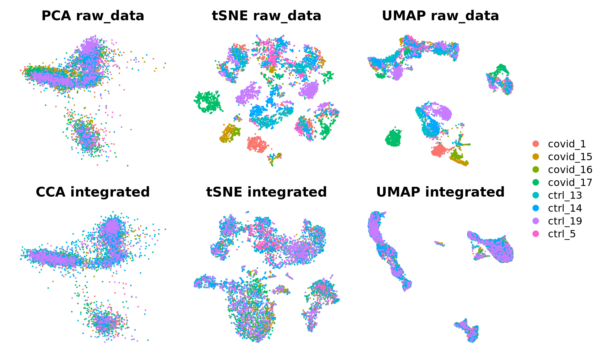
2.1 Marker genes
Let’s plot some marker genes for different cell types onto the embedding.
| Markers | Cell Type |
|---|---|
| CD3E | T cells |
| CD3E CD4 | CD4+ T cells |
| CD3E CD8A | CD8+ T cells |
| GNLY, NKG7 | NK cells |
| MS4A1 | B cells |
| CD14, LYZ, CST3, MS4A7 | CD14+ Monocytes |
| FCGR3A, LYZ, CST3, MS4A7 | FCGR3A+ Monocytes |
| FCER1A, CST3 | DCs |
myfeatures <- c("CD3E", "CD4", "CD8A", "NKG7", "GNLY", "MS4A1", "CD14", "LYZ", "MS4A7", "FCGR3A", "CST3", "FCER1A")
FeaturePlot(alldata, reduction = "umap_cca", dims = 1:2, features = myfeatures, ncol = 4, order = T) & NoLegend() & NoAxes() & NoGrid()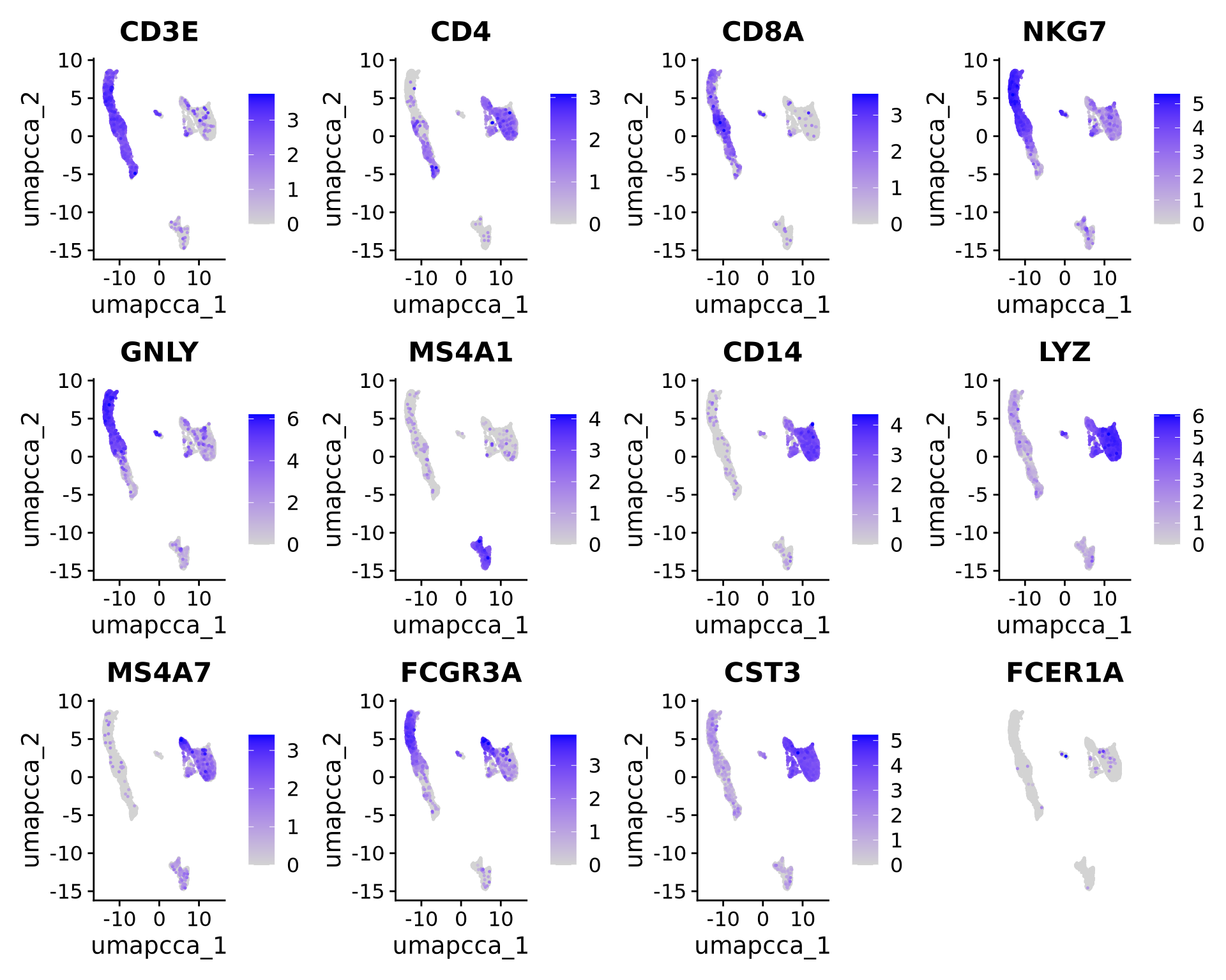
3 Harmony
An alternative method for integration is Harmony, for more details on the method, please se their paper Nat. Methods. This method runs the integration on a dimensionality reduction, in most applications the PCA. So first, we prefer to have scaling and PCA with the same set of genes that were used for the CCA integration, which we ran earlier.
We can use the same function IntegrateLayers() but intstead specify the method HarmonyIntegration. And as above, we run UMAP on the new reduction from Harmony.
alldata <- IntegrateLayers(
  object = alldata, method = HarmonyIntegration,
  orig.reduction = "pca", new.reduction = "harmony",
  verbose = FALSE
)


alldata <- RunUMAP(alldata, dims = 1:30, reduction = "harmony", reduction.name = "umap_harmony")
DimPlot(alldata, reduction = "umap_harmony", group.by = "orig.ident") + NoAxes() + ggtitle("Harmony UMAP")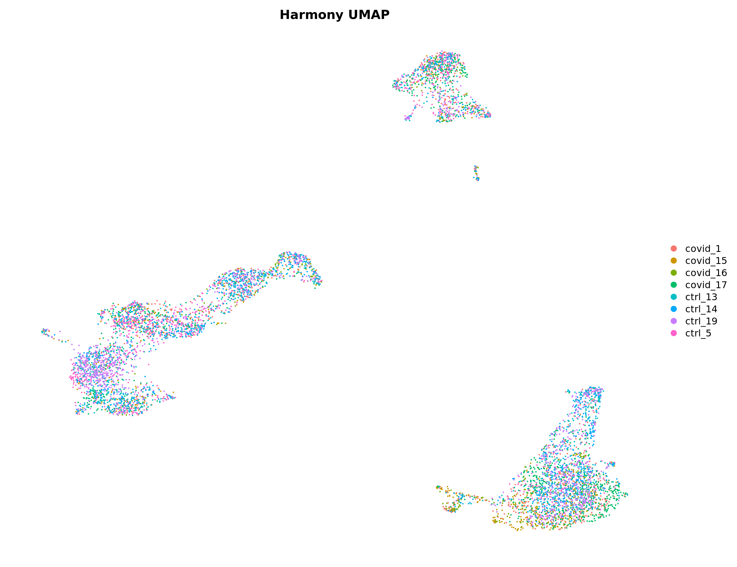
4 Scanorama
Another integration method is Scanorama (see Nat. Biotech.). This method is implemented in python, but we can run it through the Reticulate package.
We will run it with the same set of variable genes, but first we have to create a list of all the objects per sample.
Keep in mind that for most python tools that uses AnnData format the gene x cell matrix is transposed so that genes are rows and cells are columns.
# get data matrices from all samples, with only the variable genes.
data.layers <- Layers(alldata)[grep("data.",Layers(alldata))]
print(data.layers)
[1] "data.ctrl_13" "data.ctrl_14" "data.ctrl_19" "data.ctrl_5"
[5] "data.covid_15" "data.covid_16" "data.covid_17" "data.covid_1" assaylist <- lapply(data.layers, function(x) t(as.matrix(LayerData(alldata, layer = x)[hvgs_all,])))
genelist = rep(list(hvgs_all),length(assaylist))
lapply(assaylist,dim)[[1]]
[1] 1126 2000
[[2]]
[1] 1020 2000
[[3]]
[1] 1123 2000
[[4]]
[1] 1010 2000
[[5]]
[1] 575 2000
[[6]]
[1] 358 2000
[[7]]
[1] 1057 2000
[[8]]
[1] 864 2000Scanorama is implemented in python, but through reticulate we can load python packages and run python functions. In this case we also use the basilisk package for a more clean activation of python environment.
At the top of this script, we set the variable condapath to point to the conda environment where scanorama is included.
# run scanorama via basilisk with assaylis and genelist as input.
integrated.data = basiliskRun(env=condapath, fun=function(datas, genes) {
  scanorama <- reticulate::import("scanorama")
  output <- scanorama$integrate(datasets_full = datas,
                                         genes_list = genes )
  return(output)
}, datas = assaylist, genes = genelist, testload="scanorama")
Found 2000 genes among all datasets
[[0. 0.76642984 0.46393589 0.7950495 0.24869565 0.39944134
0.04446547 0.32175926]
[0. 0. 0.61887801 0.66435644 0.32869565 0.3603352
0.10690634 0.38078704]
[0. 0. 0. 0.40990099 0.36695652 0.30167598
0.21193232 0.18981481]
[0. 0. 0. 0. 0.46534653 0.44413408
0.23366337 0.55445545]
[0. 0. 0. 0. 0. 0.7877095
0.38608696 0.36695652]
[0. 0. 0. 0. 0. 0.
0.17597765 0.7122905 ]
[0. 0. 0. 0. 0. 0.
0. 0.256386 ]
[0. 0. 0. 0. 0. 0.
0. 0. ]]
Processing datasets (0, 3)
Processing datasets (4, 5)
Processing datasets (0, 1)
Processing datasets (5, 7)
Processing datasets (1, 3)
Processing datasets (1, 2)
Processing datasets (3, 7)
Processing datasets (3, 4)
Processing datasets (0, 2)
Processing datasets (3, 5)
Processing datasets (2, 3)
Processing datasets (0, 5)
Processing datasets (4, 6)
Processing datasets (1, 7)
Processing datasets (4, 7)
Processing datasets (2, 4)
Processing datasets (1, 5)
Processing datasets (1, 4)
Processing datasets (0, 7)
Processing datasets (2, 5)
Processing datasets (6, 7)
Processing datasets (0, 4)
Processing datasets (3, 6)
Processing datasets (2, 6)
Processing datasets (2, 7)
Processing datasets (5, 6)
Processing datasets (1, 6)# Now we create a new dim reduction object in the format that Seurat uses
intdimred <- do.call(rbind, integrated.data[[1]])
colnames(intdimred) <- paste0("Scanorama_", 1:100)
rownames(intdimred) <- colnames(alldata)
# Add standard deviations in order to draw Elbow Plots in Seurat
stdevs <- apply(intdimred, MARGIN = 2, FUN = sd)
# Create a new dim red object.
alldata[["scanorama"]] <- CreateDimReducObject(
embeddings = intdimred,
stdev = stdevs,
key = "Scanorama_",
assay = "RNA")Try the same but using counts instead of data.
# get count matrices from all samples, with only the variable genes.
count.layers <- Layers(alldata)[grep("counts.",Layers(alldata))]
print(count.layers)
[1] "counts.ctrl_13" "counts.ctrl_14" "counts.ctrl_19" "counts.ctrl_5"
[5] "counts.covid_15" "counts.covid_16" "counts.covid_17" "counts.covid_1" assaylist <- lapply(count.layers, function(x) t(as.matrix(LayerData(alldata, layer = x)[hvgs_all,])))
# run scanorama via basilisk with assaylis and genelist as input.
integrated.data = basiliskRun(env=condapath, fun=function(datas, genes) {
scanorama <- reticulate::import("scanorama")
output <- scanorama$integrate(datasets_full = datas,
genes_list = genes )
return(output)
}, datas = assaylist, genes = genelist, testload="scanorama")Found 2000 genes among all datasets
[[0. 0.81172291 0.65271594 0.65346535 0.18434783 0.32402235
0.10301954 0.44328704]
[0. 0. 0.66073019 0.68019802 0.25043478 0.30446927
0.15 0.46990741]
[0. 0. 0. 0.45859305 0.35173642 0.42458101
0.34817453 0.27159394]
[0. 0. 0. 0. 0.29043478 0.36312849
0.28910891 0.51089109]
[0. 0. 0. 0. 0. 0.71478261
0.62956522 0.30434783]
[0. 0. 0. 0. 0. 0.
0.51396648 0.53631285]
[0. 0. 0. 0. 0. 0.
0. 0.3125 ]
[0. 0. 0. 0. 0. 0.
0. 0. ]]
Processing datasets (0, 1)
Processing datasets (4, 5)
Processing datasets (1, 3)
Processing datasets (1, 2)
Processing datasets (0, 3)
Processing datasets (0, 2)
Processing datasets (4, 6)
Processing datasets (5, 7)
Processing datasets (5, 6)
Processing datasets (3, 7)
Processing datasets (1, 7)
Processing datasets (2, 3)
Processing datasets (0, 7)
Processing datasets (2, 5)
Processing datasets (3, 5)
Processing datasets (2, 4)
Processing datasets (2, 6)
Processing datasets (0, 5)
Processing datasets (6, 7)
Processing datasets (1, 5)
Processing datasets (4, 7)
Processing datasets (3, 4)
Processing datasets (3, 6)
Processing datasets (2, 7)
Processing datasets (1, 4)
Processing datasets (0, 4)
Processing datasets (1, 6)
Processing datasets (0, 6)# Now we create a new dim reduction object in the format that Seurat uses
# The scanorama output has 100 dimensions.
intdimred <- do.call(rbind, integrated.data[[1]])
colnames(intdimred) <- paste0("Scanorama_", 1:100)
rownames(intdimred) <- colnames(alldata)
# Add standard deviations in order to draw Elbow Plots in Seurat
stdevs <- apply(intdimred, MARGIN = 2, FUN = sd)
# Create a new dim red object.
alldata[["scanoramaC"]] <- CreateDimReducObject(
embeddings = intdimred,
stdev = stdevs,
key = "Scanorama_",
assay = "RNA")#Here we use all PCs computed from Scanorama for UMAP calculation
alldata <- RunUMAP(alldata, dims = 1:100, reduction = "scanorama",reduction.name = "umap_scanorama")
alldata <- RunUMAP(alldata, dims = 1:100, reduction = "scanoramaC",reduction.name = "umap_scanoramaC")
p1 = DimPlot(alldata, reduction = "umap_scanorama", group.by = "orig.ident") + NoAxes() + ggtitle("Scanorama UMAP")
p2 = DimPlot(alldata, reduction = "umap_scanoramaC", group.by = "orig.ident") + NoAxes() + ggtitle("ScanoramaC UMAP")
wrap_plots(p1,p2)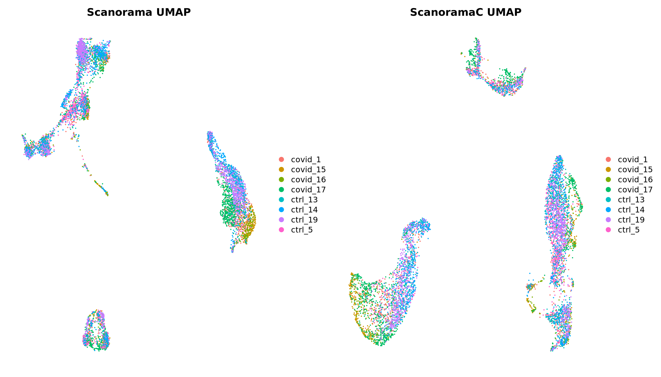
5 Overview all methods
Now we will plot UMAPS with all three integration methods side by side.
p1 <- DimPlot(alldata, reduction = "umap", group.by = "orig.ident",
              shuffle = TRUE) + ggtitle("UMAP raw_data")
p2 <- DimPlot(alldata, reduction = "umap_cca", group.by = "orig.ident",
              shuffle = TRUE) + ggtitle("UMAP CCA")
p3 <- DimPlot(alldata, reduction = "umap_harmony", group.by = "orig.ident",
              shuffle = TRUE) + ggtitle("UMAP Harmony")
p4 <- DimPlot(alldata, reduction = "umap_scanorama", group.by = "orig.ident",
              shuffle = TRUE)+ggtitle("UMAP Scanorama")

wrap_plots(p1, p2, p3, p4, nrow = 2) + plot_layout(guides = "collect")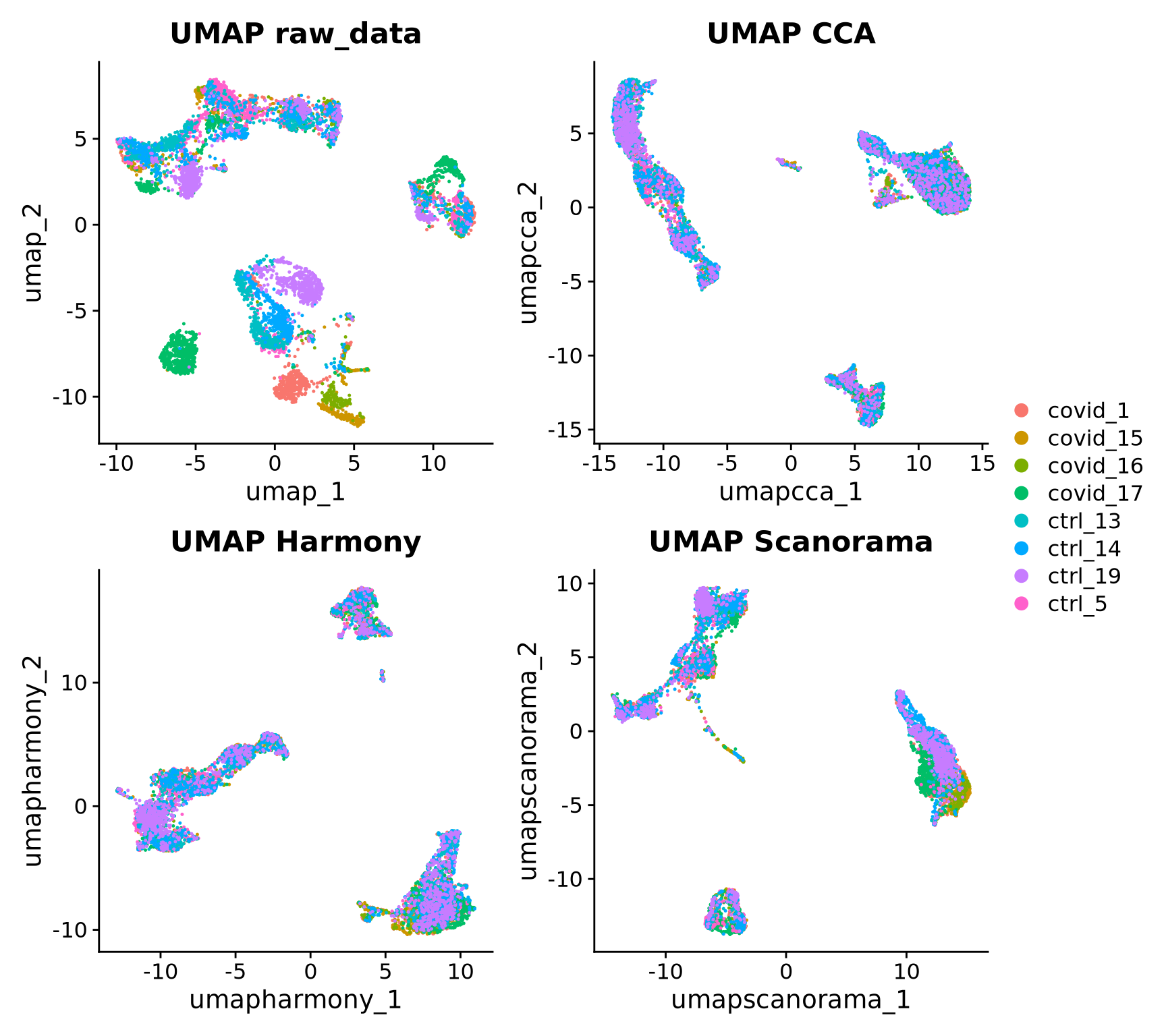
Discuss
Look at the different integration results, which one do you think looks the best? How would you motivate selecting one method over the other? How do you think you could best evaluate if the integration worked well?
Let’s save the integrated data for further analysis.
saveRDS(alldata,"data/covid/results/seurat_covid_qc_dr_int.rds")6 Extra task
You have now done the Seurat integration with CCA which is quite slow. There are other options in the IntegrateLayers() function. Try rerunning the integration with RPCAIntegration and create a new UMAP. Compare the results.
7 Session info
Click here
sessionInfo()R version 4.3.3 (2024-02-29)
Platform: x86_64-conda-linux-gnu (64-bit)
Running under: Ubuntu 20.04.6 LTS
Matrix products: default
BLAS/LAPACK: /usr/local/conda/envs/seurat/lib/libopenblasp-r0.3.28.so; LAPACK version 3.12.0
locale:
[1] LC_CTYPE=en_US.UTF-8 LC_NUMERIC=C
[3] LC_TIME=en_US.UTF-8 LC_COLLATE=en_US.UTF-8
[5] LC_MONETARY=en_US.UTF-8 LC_MESSAGES=en_US.UTF-8
[7] LC_PAPER=en_US.UTF-8 LC_NAME=C
[9] LC_ADDRESS=C LC_TELEPHONE=C
[11] LC_MEASUREMENT=en_US.UTF-8 LC_IDENTIFICATION=C
time zone: Etc/UTC
tzcode source: system (glibc)
attached base packages:
[1] stats graphics grDevices utils datasets methods base
other attached packages:
[1] basilisk_1.14.1 patchwork_1.3.0 ggplot2_3.5.1 Seurat_5.1.0
[5] SeuratObject_5.0.2 sp_2.2-0
loaded via a namespace (and not attached):
[1] deldir_2.0-4 pbapply_1.7-2 gridExtra_2.3
[4] rlang_1.1.5 magrittr_2.0.3 RcppAnnoy_0.0.22
[7] spatstat.geom_3.3-5 matrixStats_1.5.0 ggridges_0.5.6
[10] compiler_4.3.3 dir.expiry_1.10.0 png_0.1-8
[13] vctrs_0.6.5 reshape2_1.4.4 stringr_1.5.1
[16] pkgconfig_2.0.3 fastmap_1.2.0 labeling_0.4.3
[19] promises_1.3.2 rmarkdown_2.29 purrr_1.0.2
[22] xfun_0.50 jsonlite_1.8.9 goftest_1.2-3
[25] later_1.4.1 spatstat.utils_3.1-2 irlba_2.3.5.1
[28] parallel_4.3.3 cluster_2.1.8 R6_2.6.1
[31] ica_1.0-3 stringi_1.8.4 RColorBrewer_1.1-3
[34] spatstat.data_3.1-4 reticulate_1.40.0 parallelly_1.42.0
[37] spatstat.univar_3.1-1 lmtest_0.9-40 scattermore_1.2
[40] Rcpp_1.0.14 knitr_1.49 tensor_1.5
[43] future.apply_1.11.3 zoo_1.8-12 sctransform_0.4.1
[46] httpuv_1.6.15 Matrix_1.6-5 splines_4.3.3
[49] igraph_2.0.3 tidyselect_1.2.1 abind_1.4-5
[52] yaml_2.3.10 spatstat.random_3.3-2 codetools_0.2-20
[55] miniUI_0.1.1.1 spatstat.explore_3.3-4 listenv_0.9.1
[58] lattice_0.22-6 tibble_3.2.1 plyr_1.8.9
[61] basilisk.utils_1.14.1 withr_3.0.2 shiny_1.10.0
[64] ROCR_1.0-11 evaluate_1.0.3 Rtsne_0.17
[67] future_1.34.0 fastDummies_1.7.5 survival_3.8-3
[70] polyclip_1.10-7 fitdistrplus_1.2-2 filelock_1.0.3
[73] pillar_1.10.1 KernSmooth_2.23-26 plotly_4.10.4
[76] generics_0.1.3 RcppHNSW_0.6.0 munsell_0.5.1
[79] scales_1.3.0 globals_0.16.3 xtable_1.8-4
[82] RhpcBLASctl_0.23-42 glue_1.8.0 pheatmap_1.0.12
[85] lazyeval_0.2.2 tools_4.3.3 data.table_1.16.4
[88] RSpectra_0.16-2 RANN_2.6.2 leiden_0.4.3.1
[91] dotCall64_1.2 cowplot_1.1.3 grid_4.3.3
[94] tidyr_1.3.1 colorspace_2.1-1 nlme_3.1-167
[97] cli_3.6.4 spatstat.sparse_3.1-0 spam_2.11-1
[100] viridisLite_0.4.2 dplyr_1.1.4 uwot_0.2.2
[103] gtable_0.3.6 digest_0.6.37 progressr_0.15.1
[106] ggrepel_0.9.6 htmlwidgets_1.6.4 farver_2.1.2
[109] htmltools_0.5.8.1 lifecycle_1.0.4 httr_1.4.7
[112] mime_0.12 harmony_1.2.1 MASS_7.3-60.0.1