Celltype prediction

Note

Code chunks run Python commands unless it starts with %%bash, in which case, those chunks run shell commands.

Celltype prediction can either be performed on indiviudal cells where each cell gets a predicted celltype label, or on the level of clusters. All methods are based on similarity to other datasets, single cell or sorted bulk RNAseq, or uses known marker genes for each cell type.
Ideally celltype predictions should be run on each sample separately and not using the integrated data. In this case we will select one sample from the Covid data, ctrl_13 and predict celltype by cell on that sample.
Some methods will predict a celltype to each cell based on what it is most similar to, even if that celltype is not included in the reference. Other methods include an uncertainty so that cells with low similarity scores will be unclassified.
There are multiple different methods to predict celltypes, here we will just cover a few of those.

Here we will use a reference PBMC dataset that we get from scanpy datasets and classify celltypes based on two methods:

• Using scanorama for integration just as in the integration lab, and then do label transfer based on closest neighbors.
• Using ingest to project the data onto the reference data and transfer labels.
• Using Celltypist to predicted with a pretrained pbmc model or with an own model based on the same reference data as the other methods.

First, lets load required libraries

import numpy as np
import pandas as pd
import scanpy as sc
import matplotlib.pyplot as plt
import warnings
import os
import subprocess

warnings.simplefilter(action="ignore", category=Warning)

# verbosity: errors (0), warnings (1), info (2), hints (3)
sc.settings.verbosity = 2
sc.settings.set_figure_params(dpi=80)

Let’s read in the saved Covid-19 data object from the clustering step.

# download pre-computed data if missing or long compute

import requests
from urllib.parse import urljoin
from tqdm.auto import tqdm

path_data = "https://nextcloud.dc.scilifelab.se/public.php/webdav/"
auth_credentials = ("zbC5fr2LbEZ9rSE", "scRNAseq2025")

def download_file(url, destination_path, auth=None):
    
    if os.path.exists(destination_path):
        print(f"File already exists: '{destination_path}'. Skipping download.")
        return

    # Ensure the target directory exists before writing
    os.makedirs(os.path.dirname(destination_path), exist_ok=True)
    
    print(f"Initiating download for {url}...")
    
    try:
        with requests.get(url, auth=auth, stream=True) as response:
            response.raise_for_status() # Check for HTTP errors
            
            total_size = int(response.headers.get('content-length', 0))
            filename = os.path.basename(destination_path)
            
            with open(destination_path, 'wb') as f:
                with tqdm(total=total_size, unit='iB', unit_scale=True, desc=filename) as pbar:
                    for chunk in response.iter_content(chunk_size=8192):
                        if chunk:
                            f.write(chunk)
                            pbar.update(len(chunk))
                            
        print(f"Successfully downloaded: {filename}\n")
        
    except Exception as e:
        # Cleanup on failure
        if os.path.exists(destination_path):
            os.remove(destination_path)
            print(f"Cleaned up incomplete file: {destination_path}")
        print(f"Download failed due to: {e}\n")
        raise 

# Download the HDF5 file
h5ad_url = urljoin(path_data, "covid/results_scanpy/scanpy_covid_qc_dr_int_cl.h5ad")
h5ad_path = "data/covid/results/scanpy_covid_qc_dr_int_cl.h5ad"
download_file(url=h5ad_url, destination_path=h5ad_path, auth=auth_credentials)

print("Loading data into Scanpy...")
adata = sc.read_h5ad(h5ad_path)
print(adata)

File already exists: 'data/covid/results/scanpy_covid_qc_dr_int_cl.h5ad'. Skipping download.
Loading data into Scanpy...
AnnData object with n_obs × n_vars = 7222 × 4268
    obs: 'type', 'sample', 'batch', 'n_genes_by_counts', 'total_counts', 'total_counts_mt', 'pct_counts_mt', 'total_counts_ribo', 'pct_counts_ribo', 'total_counts_hb', 'pct_counts_hb', 'percent_mt2', 'n_counts', 'n_genes', 'percent_chrY', 'XIST-counts', 'S_score', 'G2M_score', 'phase', 'doublet_scores', 'predicted_doublets', 'doublet_info', 'leiden', 'leiden_0.4', 'leiden_0.6', 'leiden_1.0', 'leiden_1.4', 'kmeans5', 'kmeans10', 'kmeans15', 'hclust_5', 'hclust_10', 'hclust_15'
    var: 'gene_ids', 'feature_types', 'genome', 'mt', 'ribo', 'hb', 'n_cells_by_counts', 'mean_counts', 'pct_dropout_by_counts', 'total_counts', 'n_cells', 'highly_variable', 'means', 'dispersions', 'dispersions_norm', 'highly_variable_nbatches', 'highly_variable_intersection', 'mean', 'std'
    uns: 'dendrogram_leiden_0.6', 'doublet_info_colors', 'hclust_10_colors', 'hclust_15_colors', 'hclust_5_colors', 'hvg', 'kmeans10_colors', 'kmeans15_colors', 'kmeans5_colors', 'leiden', 'leiden_0.4', 'leiden_0.4_colors', 'leiden_0.6', 'leiden_0.6_colors', 'leiden_1.0', 'leiden_1.0_colors', 'leiden_1.4', 'leiden_1.4_colors', 'log1p', 'neighbors', 'pca', 'phase_colors', 'sample_colors', 'tsne', 'umap'
    obsm: 'Scanorama', 'X_pca', 'X_pca_combat', 'X_pca_harmony', 'X_tsne', 'X_tsne_bbknn', 'X_tsne_combat', 'X_tsne_harmony', 'X_tsne_scanorama', 'X_tsne_uncorr', 'X_umap', 'X_umap_bbknn', 'X_umap_combat', 'X_umap_harmony', 'X_umap_scanorama', 'X_umap_uncorr'
    varm: 'PCs'
    obsp: 'connectivities', 'distances'

adata.uns['log1p']['base']=None
print(adata.shape)
# have only variable genes in X, use raw instead.
adata = adata.raw.to_adata()
print(adata.shape)

(7222, 4268)
(7222, 19468)

Subset one patient.

adata = adata[adata.obs["sample"] == "ctrl_13",:]
print(adata.shape)

(1121, 19468)

adata.obs["leiden_0.6"].value_counts()

leiden_0.6
1     273
0     220
3     211
5     126
2     123
4      65
6      33
7      25
10     21
8      19
9       5
Name: count, dtype: int64

Some clusters have very few cells from this individual, so any cluster comparisons may be biased by this.

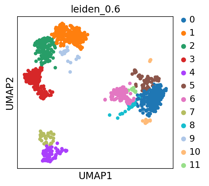
sc.pl.umap(
    adata, color=["leiden_0.6"], palette=sc.pl.palettes.default_20
)

1 Reference data

Load the reference data from scanpy.datasets. It is the annotated and processed pbmc3k dataset from 10x.

adata_ref = sc.datasets.pbmc3k_processed() 

adata_ref.obs['sample']='pbmc3k'

print(adata_ref.shape)
adata_ref.obs

(2638, 1838)

	n_genes	percent_mito	n_counts	louvain	sample
index
AAACATACAACCAC-1	781	0.030178	2419.0	CD4 T cells	pbmc3k
AAACATTGAGCTAC-1	1352	0.037936	4903.0	B cells	pbmc3k
AAACATTGATCAGC-1	1131	0.008897	3147.0	CD4 T cells	pbmc3k
AAACCGTGCTTCCG-1	960	0.017431	2639.0	CD14+ Monocytes	pbmc3k
AAACCGTGTATGCG-1	522	0.012245	980.0	NK cells	pbmc3k
...	...	...	...	...	...
TTTCGAACTCTCAT-1	1155	0.021104	3459.0	CD14+ Monocytes	pbmc3k
TTTCTACTGAGGCA-1	1227	0.009294	3443.0	B cells	pbmc3k
TTTCTACTTCCTCG-1	622	0.021971	1684.0	B cells	pbmc3k
TTTGCATGAGAGGC-1	454	0.020548	1022.0	B cells	pbmc3k
TTTGCATGCCTCAC-1	724	0.008065	1984.0	CD4 T cells	pbmc3k

2638 rows × 5 columns

As you can see, the celltype annotation is in the metadata column louvain, so that is the column we will have to use for classification.

sc.pl.umap(adata_ref, color='louvain')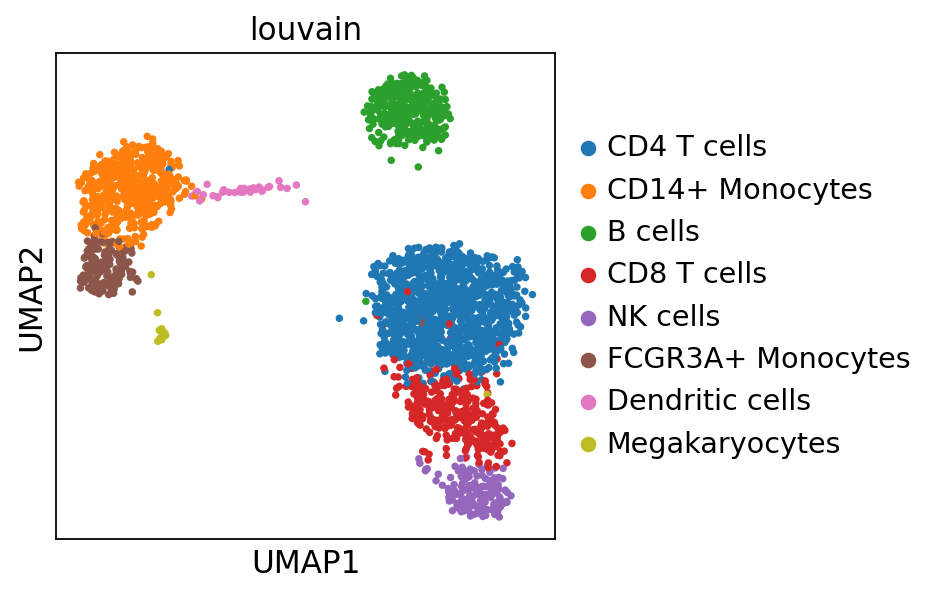

Make sure we have the same genes in both datset by taking the intersection

# before filtering genes, store the full matrix in raw.
adata.raw = adata
# also store the umap in a new slot as it will get overwritten
adata.obsm["X_umap_uncorr"] = adata.obsm["X_umap"]

print(adata_ref.shape[1])
print(adata.shape[1])
var_names = adata_ref.var_names.intersection(adata.var_names)
print(len(var_names))

adata_ref = adata_ref[:, var_names]
adata = adata[:, var_names]

1838
19468
1676

First we need to rerun pca and umap with the same gene set for both datasets.

sc.pp.pca(adata_ref, random_state=573)
sc.pp.neighbors(adata_ref, random_state=159)
sc.tl.umap(adata_ref, random_state=331)
sc.pl.umap(adata_ref, color='louvain')

computing PCA
    with n_comps=50
    finished (0:00:00)
computing neighbors
    using 'X_pca' with n_pcs = 50
    finished (0:00:04)
computing UMAP
    finished (0:00:04)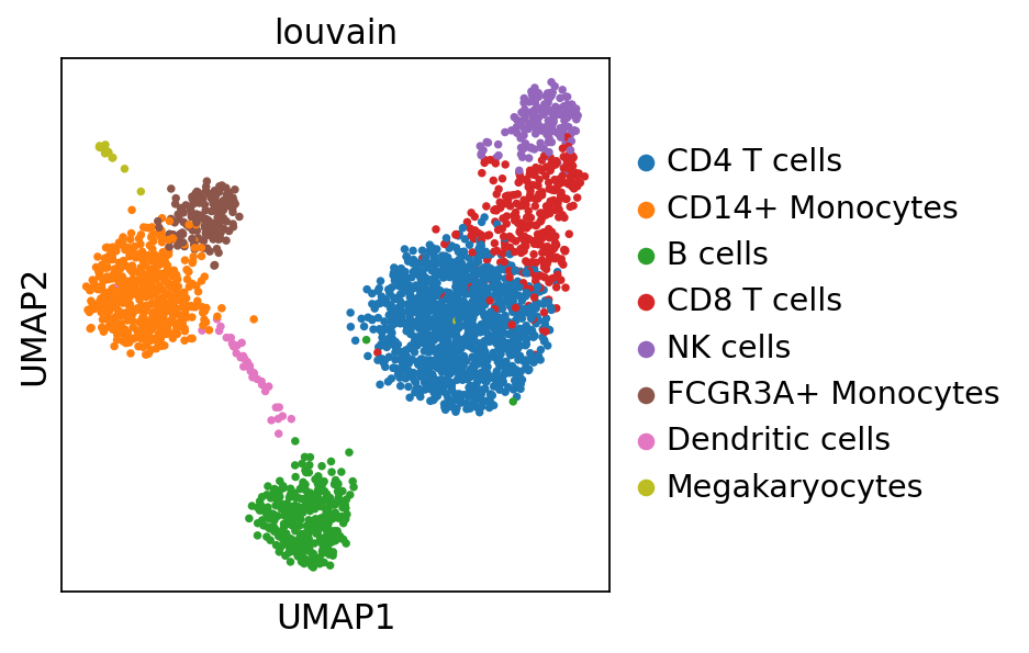

sc.pp.pca(adata, random_state=573)
sc.pp.neighbors(adata, random_state=159)
sc.tl.umap(adata, random_state=331)
sc.pl.umap(adata, color='leiden_0.6')

computing PCA
    with n_comps=50
    finished (0:00:00)
computing neighbors
    using 'X_pca' with n_pcs = 50
    finished (0:00:00)
computing UMAP
    finished (0:00:01)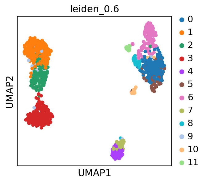

2 Integrate with scanorama

import scanorama

#subset the individual dataset to the same variable genes as in MNN-correct.
alldata = dict()
alldata['ctrl']=adata
alldata['ref']=adata_ref

#convert to list of AnnData objects
adatas = list(alldata.values())

# run scanorama.integrate
scanorama.integrate_scanpy(adatas, dimred = 50)

Found 1676 genes among all datasets
[[0.         0.49509367]
 [0.         0.        ]]
Processing datasets (0, 1)

# add in sample info
adata_ref.obs['sample']='pbmc3k'

# create a merged scanpy object and add in the scanorama 
adata_merged = alldata['ctrl'].concatenate(alldata['ref'], batch_key='sample', batch_categories=['ctrl','pbmc3k'])

embedding = np.concatenate([ad.obsm['X_scanorama'] for ad in adatas], axis=0)
adata_merged.obsm['Scanorama'] = embedding

#run  umap.
sc.pp.neighbors(adata_merged, n_pcs =50, use_rep = "Scanorama", random_state=159)
sc.tl.umap(adata_merged, random_state=331)

computing neighbors
    finished (0:00:00)
computing UMAP
    finished (0:00:04)

sc.pl.umap(adata_merged, color=["sample","louvain"])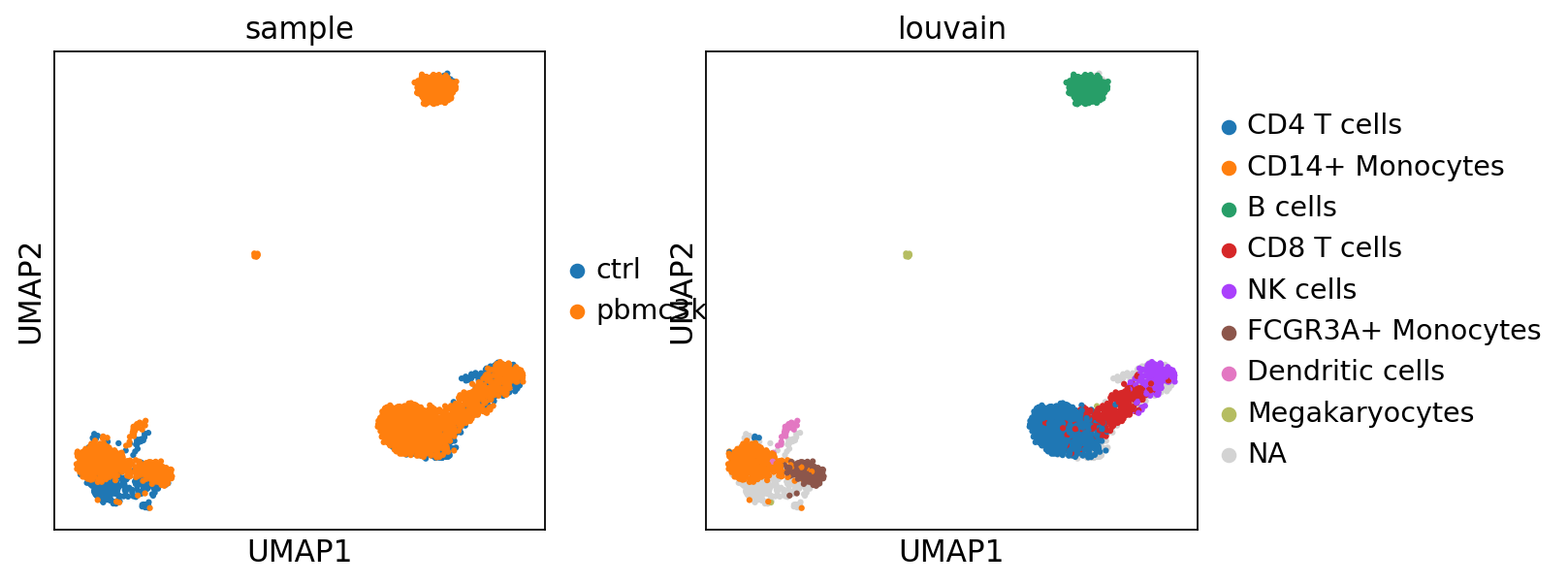

2.1 Label transfer

Using the functions from the Spatial tutorial from Scanpy we will calculate normalized cosine distances between the two datasets and tranfer labels to the celltype with the highest scores.

from sklearn.metrics.pairwise import cosine_distances

distances = 1 - cosine_distances(
    adata_merged[adata_merged.obs['sample'] == "pbmc3k"].obsm["Scanorama"],
    adata_merged[adata_merged.obs['sample'] == "ctrl"].obsm["Scanorama"],
)

def label_transfer(dist, labels, index):
    lab = pd.get_dummies(labels)
    class_prob = lab.to_numpy().T @ dist
    norm = np.linalg.norm(class_prob, 2, axis=0)
    class_prob = class_prob / norm
    class_prob = (class_prob.T - class_prob.min(1)) / np.ptp(class_prob, 1)
    # convert to df
    cp_df = pd.DataFrame(
        class_prob, columns=lab.columns
    )
    cp_df.index = index
    # classify as max score
    m = cp_df.idxmax(axis=1)
    
    return m

class_def = label_transfer(distances, adata_ref.obs.louvain, adata.obs.index)

# add to obs section of the original object
adata.obs['label_trans'] = class_def

sc.pl.umap(adata, color="label_trans")

# add to merged object.
adata_merged.obs["label_trans"] = pd.concat(
    [class_def, adata_ref.obs["louvain"]], axis=0
).tolist()

sc.pl.umap(adata_merged, color=["sample","louvain",'label_trans'])
#plot only ctrl cells.
sc.pl.umap(adata_merged[adata_merged.obs['sample']=='ctrl'], color='label_trans')

Now plot how many cells of each celltypes can be found in each cluster.

tmp = pd.crosstab(adata.obs['leiden_0.6'],adata.obs['label_trans'], normalize='index')
tmp.plot.bar(stacked=True).legend(bbox_to_anchor=(1.8, 1),loc='upper right')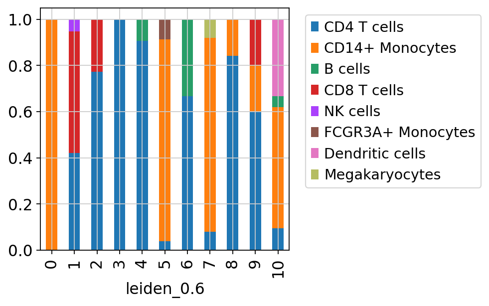

3 Ingest

Another method for celltype prediction is Ingest, for more information, please look at https://scanpy-tutorials.readthedocs.io/en/latest/integrating-data-using-ingest.html

sc.tl.ingest(adata, adata_ref, obs='louvain')
sc.pl.umap(adata, color=['louvain','leiden_0.6'], wspace=0.5)

running ingest
    finished (0:00:15)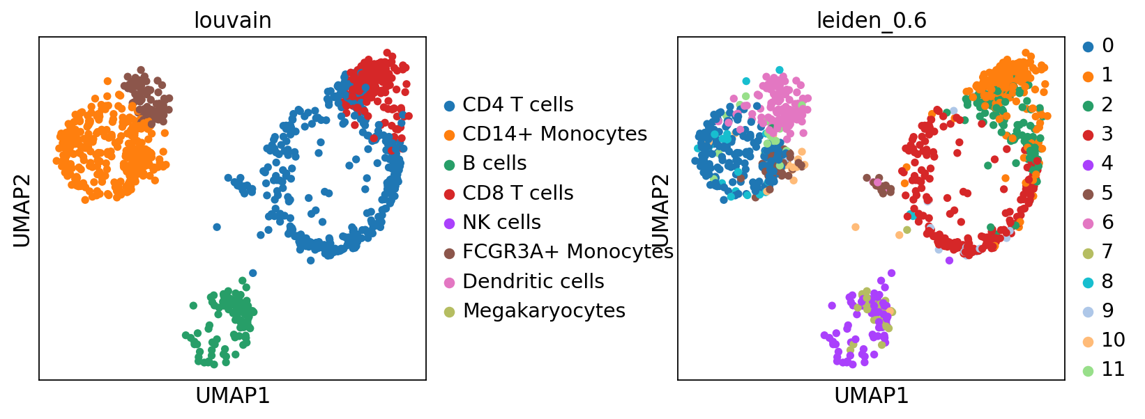

As you can see, ingest has created a new umap for us, so to get consistent plotting, lets revert back to the old one for further plotting:

adata.obsm["X_umap"] = adata.obsm["X_umap_uncorr"]

sc.pl.umap(adata, color=['louvain','leiden_0.6'], wspace=0.5)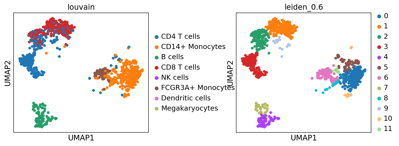

Now plot how many cells of each celltypes can be found in each cluster.

tmp = pd.crosstab(adata.obs['leiden_0.6'],adata.obs['louvain'], normalize='index')
tmp.plot.bar(stacked=True).legend(bbox_to_anchor=(1.8, 1),loc='upper right')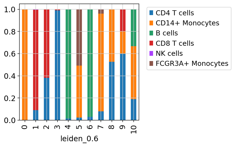

4 Celltypist

Celltypist provides pretrained models for classification for many different human tissues and celltypes. Here, we are following the steps of this tutorial, with some adaptations for this dataset. So please check out the tutorial for more detail.

import celltypist
from celltypist import models

# there are many different models, we will only download 2 of them for now.
models.download_models(force_update = False, model = 'Immune_All_Low.pkl')
models.download_models(force_update = False, model = 'Immune_All_High.pkl')

Now select the model you want to use and show the info:

model = models.Model.load(model = 'Immune_All_High.pkl')

model

CellTypist model with 32 cell types and 6639 features
    date: 2022-07-16 08:53:00.959521
    details: immune populations combined from 20 tissues of 18 studies
    source: https://doi.org/10.1126/science.abl5197
    version: v2
    cell types: B cells, B-cell lineage, ..., pDC precursor
    features: A1BG, A2M, ..., ZYX

To infer celltype labels to our cells, we first need to convert back to the full matrix. OBS! For celltypist we want to have log1p normalised expression to 10,000 counts per cell. Which we already have in adata.raw.X, check by summing up the data, it should sum to 10K.

adata = adata.raw.to_adata() 
adata.X.expm1().sum(axis = 1)[:10]

matrix([[10000.],
        [10000.],
        [10000.],
        [10000.],
        [10000.],
        [10000.],
        [10000.],
        [10000.],
        [10000.],
        [10000.]])

predictions = celltypist.annotate(adata, model = 'Immune_All_High.pkl', majority_voting = True)

predictions.predicted_labels

running Leiden clustering
    finished (0:00:00)

	predicted_labels	over_clustering	majority_voting
AGGTCATGTGCGAACA-13-5	T cells	0	T cells
CCTATCGGTCCCTCAT-13-5	ILC	1	ILC
TCCTCCCTCGTTCATT-13-5	ILC	3	ILC
CAACCAATCATCTATC-13-5	ILC	4	ILC
TACGGTATCGGATTAC-13-5	T cells	5	T cells
...	...	...	...
TCCACCATCATAGCAC-13-5	T cells	0	T cells
GAGTTACAGTGAGTGC-13-5	T cells	19	T cells
ATCATTCAGGCTCACC-13-5	Monocytes	24	Monocytes
AGCCACGCAACCCTAA-13-5	T cells	20	T cells
CTACCTGGTCAGGAGT-13-5	ILC	10	ILC

1121 rows × 3 columns

The first column predicted_labels is the predictions made for each individual cell, while majority_voting is done for local subclusters, the clustering identities are in column over_clustering.

Now we convert the predictions to an anndata object.

adata = predictions.to_adata()

sc.pl.umap(adata, color = ['leiden_0.6', 'predicted_labels', 'majority_voting'], legend_loc = 'on data')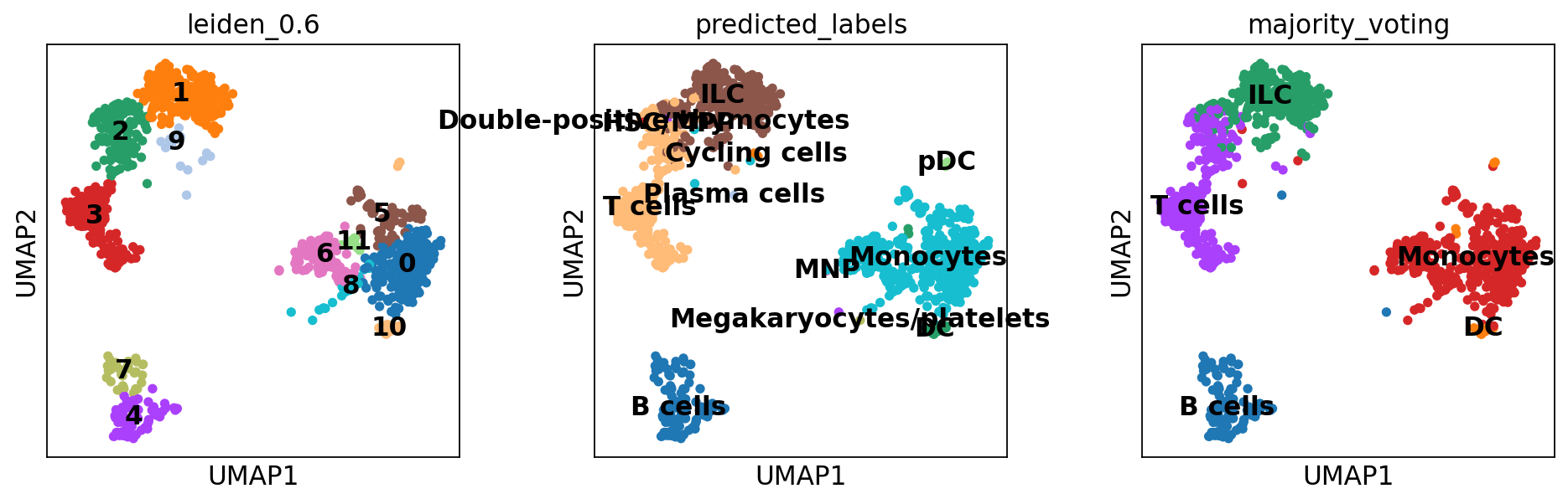

NoteTask

Rerun predictions with Celltypist, but use another model, for instance Immune_All_High.pkl, or any other model you find relevant, you can find a list of models here. How do the results differ for you?

4.1 Celltypist custom model

We can also train our own model on any reference data that we want to use. In this case we will use the pbmc data in adata_ref to train a model.

Celltypist requires the data to be in the format of log1p normalised expression to 10,000 counts per cell, we can check if that is the case for the object we have:

adata_ref.raw.X.expm1().sum(axis = 1)[:10]

matrix([[2419.],
        [4903.],
        [3147.],
        [2639.],
        [ 980.],
        [2163.],
        [2175.],
        [2260.],
        [1275.],
        [1103.]], dtype=float32)

These should all sum up to 10K, which is not the case, probably since some genes were removed after normalizing. Wo we will have to start from the raw counts of that dataset instead. Before we selected the data pbmc3k_processed, but now we will instead use pbmc3k.

adata_ref2 = sc.datasets.pbmc3k() 
adata_ref2

AnnData object with n_obs × n_vars = 2700 × 32738
    var: 'gene_ids'

This data is not annotated, so we will have to match the indices from the filtered and processed object. And add in the metadata with annotations.

adata_ref2 = adata_ref2[adata_ref.obs_names,:]
adata_ref2.obs = adata_ref.obs
adata_ref2

AnnData object with n_obs × n_vars = 2638 × 32738
    obs: 'n_genes', 'percent_mito', 'n_counts', 'louvain', 'sample'
    var: 'gene_ids'

Now we can normalize the matrix:

sc.pp.normalize_total(adata_ref2, target_sum = 1e4)
sc.pp.log1p(adata_ref2)

# check the sums again
adata_ref2.X.expm1().sum(axis = 1)[:10]

normalizing counts per cell
    finished (0:00:01)

matrix([[10000.   ],
        [10000.   ],
        [10000.   ],
        [ 9999.998],
        [ 9999.998],
        [10000.   ],
        [ 9999.999],
        [10000.   ],
        [10000.001],
        [10000.   ]], dtype=float32)

And finally train the model.

new_model = celltypist.train(adata_ref2, labels = 'louvain', n_jobs = 10, feature_selection = True)

Now we can run predictions on our data

predictions2 = celltypist.annotate(adata, model = new_model, majority_voting = True)

running Leiden clustering
    finished (0:00:00)

Instead of converting the predictions to anndata we will just add another column in the adata.obs with these new predictions since the column names from the previous celltypist runs with clash.

adata.obs["predicted_labels_ref"] = predictions2.predicted_labels["predicted_labels"]
adata.obs["majority_voting_ref"] = predictions2.predicted_labels["majority_voting"]

sc.pl.umap(adata, color = ['predicted_labels', 'majority_voting','predicted_labels_ref', 'majority_voting_ref'], legend_loc = 'on data', ncols=2)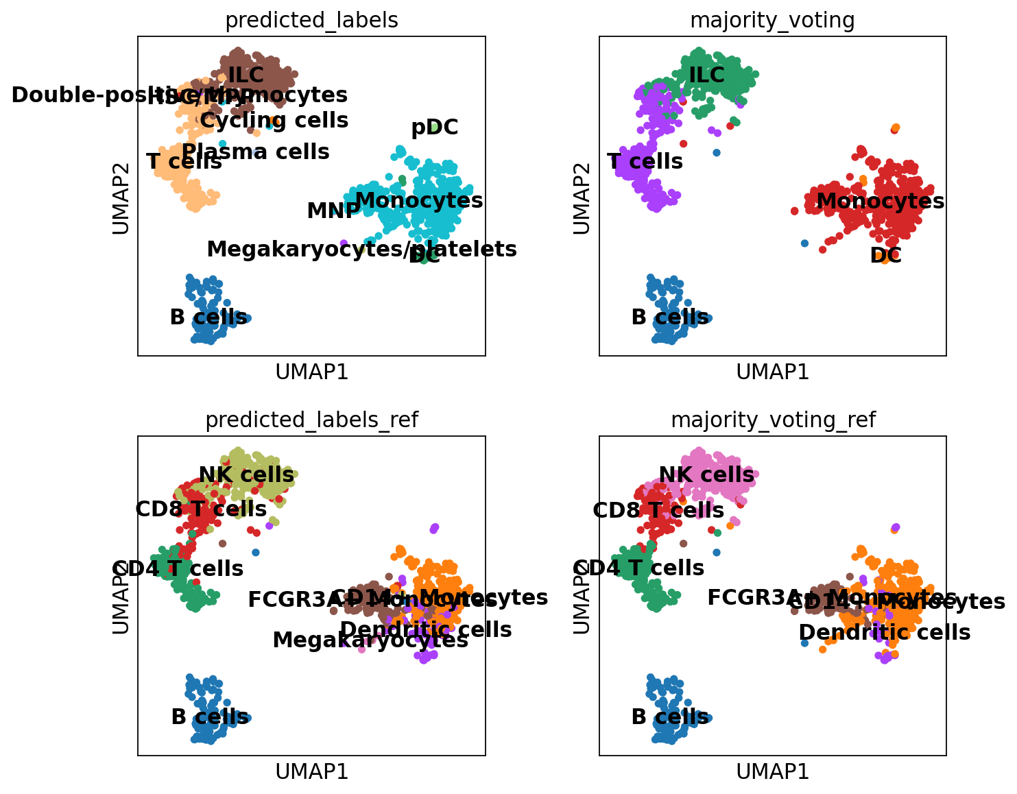

5 Compare results

The predictions from ingest is stored in the column ‘louvain’ while we named the label transfer with scanorama as ‘predicted’

sc.pl.umap(adata, color=['louvain','label_trans','majority_voting', 'majority_voting_ref'], wspace=0.5, ncols=3)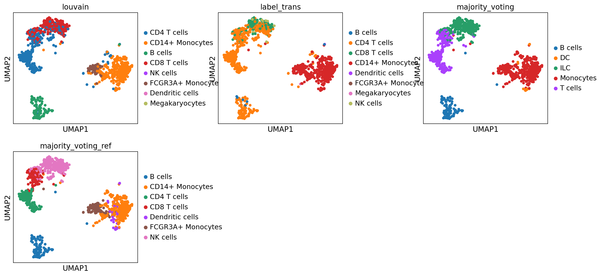

As you can see, the main celltypes are generally the same, but there are clearly differences, especially with regards to the cells predicted as either ILC/NK/CD8 T-cells.

The only way to make sure which method you trust is to look at what genes the different celltypes express and use your biological knowledge to make decisions.

6 Gene set analysis

Another way of predicting celltypes is to use the differentially expressed genes per cluster and compare to lists of known cell marker genes. This requires a list of genes that you trust and that is relevant for the tissue you are working on.

You can either run it with a marker list from the ontology or a list of your choice as in the example below.

markers_url = urljoin(path_data, "misc/human_cell_markers.txt")
markers_path = "data/human_cell_markers.txt"
download_file(url=markers_url, destination_path=markers_path, auth=auth_credentials)

File already exists: 'data/human_cell_markers.txt'. Skipping download.

print("Loading data...")
df = pd.read_table(markers_path)
print(df.shape)

Loading data...
(2868, 15)

# Filter for number of genes per celltype
df['nG'] = df.geneSymbol.str.split(",").str.len()

df = df[df['nG'] > 5]
df = df[df['nG'] < 100]
d = df[df['cancerType'] == "Normal"]
print(df.shape)

# convert to dict.
df.index = df.cellName
gene_dict = df.geneSymbol.str.split(",").to_dict()

(445, 16)

# run differential expression per cluster
sc.tl.rank_genes_groups(adata, 'leiden_0.6', method='wilcoxon', key_added = "wilcoxon")

ranking genes
    finished (0:00:00)

# do gene set overlap to the groups in the gene list and top 300 DEGs.

import gseapy

gsea_res = dict()
pred = dict()

for cl in adata.obs['leiden_0.6'].cat.categories:
    print(f"Processing cluster: {cl}")

    df_group = sc.get.rank_genes_groups_df(adata, group=cl, key='wilcoxon')

    if df_group.empty:
        pred[cl] = "Unass"
        continue

    glist = df_group['names'].squeeze().str.strip().tolist()
    top_genes = glist[:300]

    if not top_genes:
        pred[cl] = "Unass"
        continue

    enr_res = gseapy.enrichr(
        gene_list=top_genes,
        organism='Human',
        gene_sets=gene_dict,
        background=adata.shape[1],
        cutoff=1
    )

    results = enr_res.results

    if isinstance(results, pd.DataFrame) and not results.empty:
        # Sort by P-value, then Combined Score
        results.sort_values(
            by=["P-value", "Combined Score"], 
            ascending=[True, False], 
            inplace=True
        )
        gsea_res[cl] = enr_res

        best_p_val = results["P-value"].iloc[0]
        best_c_score = results["Combined Score"].iloc[0]

        top_hits = results[
            (results["P-value"] == best_p_val) & 
            (results["Combined Score"] == best_c_score)
        ]

        # Concatenate top hits labels
        pred[cl] = " / ".join(top_hits["Term"].tolist())
        print(f"Assigned: {pred[cl]}")

    else:
        pred[cl] = "Unass"

Processing cluster: 0
Assigned: Cancer stem-like cell / Macrophage / Myeloblast
Processing cluster: 1
Assigned: Effector T cell
Processing cluster: 2
Assigned: Monocyte / Parietal progenitor cell / T cell
Processing cluster: 3
Assigned: Effector memory T cell / Naive T cell / T cell
Processing cluster: 4
Assigned: B cell
Processing cluster: 5
Assigned: Macrophage
Processing cluster: 6
Assigned: B cell
Processing cluster: 7
Assigned: Macrophage / Myeloblast / Spermatogonial stem cell
Processing cluster: 8
Assigned: Lake et al.Science.In4 / Myeloblast / Spermatogonial stem cell
Processing cluster: 9
Assigned: Circulating fetal cell
Processing cluster: 10
Assigned: PROM1Low progenitor cell

# prediction per cluster
pred

{'0': 'Cancer stem-like cell / Macrophage / Myeloblast',
 '1': 'Effector T cell',
 '2': 'Monocyte / Parietal progenitor cell / T cell',
 '3': 'Effector memory T cell / Naive T cell / T cell',
 '4': 'B cell',
 '5': 'Macrophage',
 '6': 'B cell',
 '7': 'Macrophage / Myeloblast / Spermatogonial stem cell',
 '8': 'Lake et al.Science.In4 / Myeloblast / Spermatogonial stem cell',
 '9': 'Circulating fetal cell',
 '10': 'PROM1Low progenitor cell'}

prediction = [pred[x] for x in adata.obs['leiden_0.6']]
adata.obs["GS_overlap_pred"] = prediction

sc.pl.umap(adata, color='GS_overlap_pred')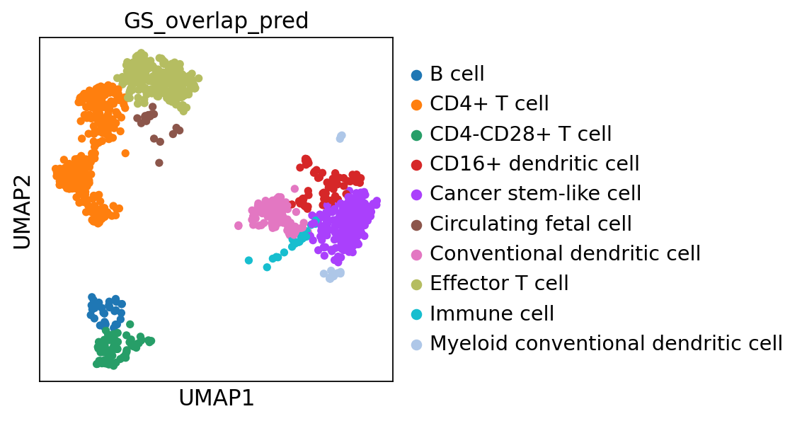

NoteDiscuss

As you can see, it agrees to some extent with the predictions from the methods above, but there are clear differences, which do you think looks better?

7 Save data

We can finally save the object for use in future steps.

adata.write_h5ad('data/covid/results/scanpy_covid_qc_dr_int_cl_ct-ctrl13.h5ad')

8 Session info

Click here

sc.logging.print_versions()

Dependencies

Dependency	Version
natsort	8.4.0
numcodecs	0.16.5
cycler	0.12.1
igraph	1.0.0
urllib3	2.6.3
array-api-compat	1.13.0
packaging	26.0
platformdirs	4.9.2
zarr	3.1.5
Brotli	1.2.0
asttokens	3.0.1
fbpca	1.0
joblib	1.5.3
charset-normalizer	3.4.4
executing	2.2.1
texttable	1.7.0
wcwidth	0.6.0
intervaltree	3.1.0
xarray	2026.2.0
jupyter_core	5.9.1
comm	0.2.3
six	1.17.0
jedi	0.19.2
llvmlite	0.46.0
sparse	0.18.0
umap-learn	0.5.11
typing_extensions	4.15.0
pure_eval	0.2.3
idna	3.11
donfig	0.8.1.post1
psutil	7.2.2
h5py	3.15.1
stack_data	0.6.3
numba	0.63.1
google-crc32c	1.8.0
session-info2	0.4
ipykernel	7.2.0
threadpoolctl	3.6.0
ipython	9.10.0
scipy	1.16.3
annoy	1.17.3
pyparsing	3.3.2
prompt_toolkit	3.0.52
PySocks	1.7.1
statsmodels	0.14.6
python-dateutil	2.9.0.post0
decorator	5.2.1
fast-array-utils	1.3.1
sortedcontainers	2.4.0
traitlets	5.14.3
fsspec	2026.2.0
jupyter_client	8.8.0
tornado	6.5.3
pytz	2025.2
pynndescent	0.5.13
msgpack	1.1.2
kiwisolver	1.4.9
Pygments	2.19.2
patsy	1.0.2
PyYAML	6.0.3
backports.zstd	1.3.0
matplotlib-inline	0.2.1
setuptools	82.0.0
parso	0.8.6
pillow	12.1.1
pyzmq	27.1.0
debugpy	1.8.20
legacy-api-wrap	1.5
certifi	2026.1.4 (2026.01.04)

Copyable Markdown

| Package      | Version |
| ------------ | ------- |
| numpy        | 2.3.5   |
| pandas       | 2.3.3   |
| scanpy       | 1.12    |
| matplotlib   | 3.10.8  |
| requests     | 2.32.5  |
| tqdm         | 4.67.3  |
| anndata      | 0.12.10 |
| scanorama    | 1.7.4   |
| scikit-learn | 1.6.1   |
| celltypist   | 1.7.1   |
| gseapy       | 1.1.11  |

| Dependency         | Version               |
| ------------------ | --------------------- |
| natsort            | 8.4.0                 |
| numcodecs          | 0.16.5                |
| cycler             | 0.12.1                |
| igraph             | 1.0.0                 |
| urllib3            | 2.6.3                 |
| array-api-compat   | 1.13.0                |
| packaging          | 26.0                  |
| platformdirs       | 4.9.2                 |
| zarr               | 3.1.5                 |
| Brotli             | 1.2.0                 |
| asttokens          | 3.0.1                 |
| fbpca              | 1.0                   |
| joblib             | 1.5.3                 |
| charset-normalizer | 3.4.4                 |
| executing          | 2.2.1                 |
| texttable          | 1.7.0                 |
| wcwidth            | 0.6.0                 |
| intervaltree       | 3.1.0                 |
| xarray             | 2026.2.0              |
| jupyter_core       | 5.9.1                 |
| comm               | 0.2.3                 |
| six                | 1.17.0                |
| jedi               | 0.19.2                |
| llvmlite           | 0.46.0                |
| sparse             | 0.18.0                |
| umap-learn         | 0.5.11                |
| typing_extensions  | 4.15.0                |
| pure_eval          | 0.2.3                 |
| idna               | 3.11                  |
| donfig             | 0.8.1.post1           |
| psutil             | 7.2.2                 |
| h5py               | 3.15.1                |
| stack_data         | 0.6.3                 |
| numba              | 0.63.1                |
| google-crc32c      | 1.8.0                 |
| session-info2      | 0.4                   |
| ipykernel          | 7.2.0                 |
| threadpoolctl      | 3.6.0                 |
| ipython            | 9.10.0                |
| scipy              | 1.16.3                |
| annoy              | 1.17.3                |
| pyparsing          | 3.3.2                 |
| prompt_toolkit     | 3.0.52                |
| PySocks            | 1.7.1                 |
| statsmodels        | 0.14.6                |
| python-dateutil    | 2.9.0.post0           |
| decorator          | 5.2.1                 |
| fast-array-utils   | 1.3.1                 |
| sortedcontainers   | 2.4.0                 |
| traitlets          | 5.14.3                |
| fsspec             | 2026.2.0              |
| jupyter_client     | 8.8.0                 |
| tornado            | 6.5.3                 |
| pytz               | 2025.2                |
| pynndescent        | 0.5.13                |
| msgpack            | 1.1.2                 |
| kiwisolver         | 1.4.9                 |
| Pygments           | 2.19.2                |
| patsy              | 1.0.2                 |
| PyYAML             | 6.0.3                 |
| backports.zstd     | 1.3.0                 |
| matplotlib-inline  | 0.2.1                 |
| setuptools         | 82.0.0                |
| parso              | 0.8.6                 |
| pillow             | 12.1.1                |
| pyzmq              | 27.1.0                |
| debugpy            | 1.8.20                |
| legacy-api-wrap    | 1.5                   |
| certifi            | 2026.1.4 (2026.01.04) |

| Component | Info                                                                           |
| --------- | ------------------------------------------------------------------------------ |
| Python    | 3.12.12 | packaged by conda-forge | (main, Jan 26 2026, 23:51:32) [GCC 14.3.0] |
| OS        | Linux-6.12.5-linuxkit-x86_64-with-glibc2.35                                    |
| CPU       | 16 logical CPU cores, x86_64                                                   |
| GPU       | No GPU found                                                                   |
| Updated   | 2026-04-17 10:26                                                               |