# BiocManager::install('DropletUtils',update = F)
# BiocManager::install("Spaniel",update = F)
# remotes::install_github("RachelQueen1/Spaniel", ref = "Development" ,upgrade = F,dependencies = F)
# remotes::install_github("renozao/xbioc")
# remotes::install_github("meichendong/SCDC")

suppressPackageStartupMessages({
    library(Spaniel)
    # library(biomaRt)
    library(SingleCellExperiment)
    library(Matrix)
    library(dplyr)
    library(scran)
    library(SingleR)
    library(scater)
    library(ggplot2)
    library(patchwork)
})
Note
Code chunks run R commands unless otherwise specified.
Spatial transcriptomic data with the Visium platform is in many ways similar to scRNAseq data. It contains UMI counts for 5-20 cells instead of single cells, but is still quite sparse in the same way as scRNAseq data is, but with the additional information about spatial location in the tissue.
Here we will first run quality control in a similar manner to scRNAseq data, then QC filtering, dimensionality reduction, integration and clustering. Then we will use scRNAseq data from mouse cortex to run label transfer to predict celltypes in the Visium spots.
We will use two Visium spatial transcriptomics dataset of the mouse brain (Sagittal), which are publicly available from the 10x genomics website. Note, that these dataset have already been filtered for spots that does not overlap with the tissue.
1 Preparation
Load packages
Load ST data
# url for source and intermediate data
path_data <- "https://export.uppmax.uu.se/naiss2023-23-3/workshops/workshop-scrnaseq"
if (!dir.exists("data/spatial/visium/Anterior")) dir.create("data/spatial/visium/Anterior", recursive = T)
if (!dir.exists("data/spatial/visium/Posterior")) dir.create("data/spatial/visium/Posterior", recursive = T)
file_list <- c(
"spatial/visium/Anterior/V1_Mouse_Brain_Sagittal_Anterior_filtered_feature_bc_matrix.tar.gz",
"spatial/visium/Anterior/V1_Mouse_Brain_Sagittal_Anterior_spatial.tar.gz",
"spatial/visium/Posterior/V1_Mouse_Brain_Sagittal_Posterior_filtered_feature_bc_matrix.tar.gz",
"spatial/visium/Posterior/V1_Mouse_Brain_Sagittal_Posterior_spatial.tar.gz"
)
for (i in file_list) {
if (!file.exists(file.path("data", i))) {
cat(paste0("Downloading ", file.path(path_data, i), " to ", file.path("data", i), "\n"))
download.file(url = file.path(path_data, i), destfile = file.path("data", i))
}
cat(paste0("Uncompressing ", file.path("data", i), "\n"))
system(paste0("tar -xvzf ", file.path("data", i), " -C ", dirname(file.path("data", i))))
}Downloading https://export.uppmax.uu.se/naiss2023-23-3/workshops/workshop-scrnaseq/spatial/visium/Anterior/V1_Mouse_Brain_Sagittal_Anterior_filtered_feature_bc_matrix.tar.gz to data/spatial/visium/Anterior/V1_Mouse_Brain_Sagittal_Anterior_filtered_feature_bc_matrix.tar.gz
Uncompressing data/spatial/visium/Anterior/V1_Mouse_Brain_Sagittal_Anterior_filtered_feature_bc_matrix.tar.gz
Downloading https://export.uppmax.uu.se/naiss2023-23-3/workshops/workshop-scrnaseq/spatial/visium/Anterior/V1_Mouse_Brain_Sagittal_Anterior_spatial.tar.gz to data/spatial/visium/Anterior/V1_Mouse_Brain_Sagittal_Anterior_spatial.tar.gz
Uncompressing data/spatial/visium/Anterior/V1_Mouse_Brain_Sagittal_Anterior_spatial.tar.gz
Downloading https://export.uppmax.uu.se/naiss2023-23-3/workshops/workshop-scrnaseq/spatial/visium/Posterior/V1_Mouse_Brain_Sagittal_Posterior_filtered_feature_bc_matrix.tar.gz to data/spatial/visium/Posterior/V1_Mouse_Brain_Sagittal_Posterior_filtered_feature_bc_matrix.tar.gz
Uncompressing data/spatial/visium/Posterior/V1_Mouse_Brain_Sagittal_Posterior_filtered_feature_bc_matrix.tar.gz
Downloading https://export.uppmax.uu.se/naiss2023-23-3/workshops/workshop-scrnaseq/spatial/visium/Posterior/V1_Mouse_Brain_Sagittal_Posterior_spatial.tar.gz to data/spatial/visium/Posterior/V1_Mouse_Brain_Sagittal_Posterior_spatial.tar.gz
Uncompressing data/spatial/visium/Posterior/V1_Mouse_Brain_Sagittal_Posterior_spatial.tar.gzMerge the objects into one SCE object.
sce.a <- Spaniel::createVisiumSCE(tenXDir = "data/spatial/visium/Anterior", resolution = "Low")
sce.p <- Spaniel::createVisiumSCE(tenXDir = "data/spatial/visium/Posterior", resolution = "Low")
sce <- cbind(sce.a, sce.p)

sce$Sample <- basename(sub("/filtered_feature_bc_matrix", "", sce$Sample))

lll <- list(sce.a, sce.p)
lll <- lapply(lll, function(x) x@metadata)
names(lll) <- c("Anterior", "Posterior")
sce@metadata <- lll
We can further convert the gene ensembl IDs to gene names using biomaRt.
mart <- biomaRt::useMart(biomart = "ENSEMBL_MART_ENSEMBL", dataset = "mmusculus_gene_ensembl")
annot <- biomaRt::getBM(attributes = c("ensembl_gene_id", "external_gene_name", "gene_biotype"), mart = mart, useCache = F)
saveRDS(annot, "data/spatial/visium/annot.rds")
We will use a file that was created in advance.
path_file <- "data/spatial/visium/annot.rds"
if (!file.exists(path_file)) download.file(url = file.path(path_data, "spatial/visium/annot.rds"), destfile = path_file)
annot <- readRDS(path_file)
gene_names <- as.character(annot[match(rownames(sce), annot[, "ensembl_gene_id"]), "external_gene_name"])
gene_names[is.na(gene_names)] <- ""
sce <- sce[gene_names != "", ]
rownames(sce) <- gene_names[gene_names != ""]
dim(sce)[1] 32053 60502 Quality control
Similar to scRNA-seq we use statistics on number of counts, number of features and percent mitochondria for quality control.
Now the counts and feature counts are calculated on the Spatial assay, so they are named nCount_Spatial and nFeature_Spatial.
# Mitochondrial genes
mito_genes <- rownames(sce)[grep("^mt-", rownames(sce))]

# Ribosomal genes
ribo_genes <- rownames(sce)[grep("^Rp[sl]", rownames(sce))]

# Hemoglobin genes - includes all genes starting with HB except HBP.
hb_genes <- rownames(sce)[grep("^Hb[^(p)]", rownames(sce))]

sce <- addPerCellQC(sce, flatten = T, subsets = list(mt = mito_genes, hb = hb_genes, ribo = ribo_genes))

head(colData(sce))
DataFrame with 6 rows and 24 columns
Sample Barcode Section Spot_Y Spot_X Image_Y
<character> <character> <integer> <integer> <integer> <integer>
1 Anterior AAACAAGTATCTCCCA-1 1 50 102 7474
2 Anterior AAACACCAATAACTGC-1 1 59 19 8552
3 Anterior AAACAGAGCGACTCCT-1 1 14 94 3163
4 Anterior AAACAGCTTTCAGAAG-1 1 43 9 6636
5 Anterior AAACAGGGTCTATATT-1 1 47 13 7115
6 Anterior AAACATGGTGAGAGGA-1 1 62 0 8912
Image_X pixel_x pixel_y sum detected total sum
<integer> <numeric> <numeric> <numeric> <integer> <numeric> <numeric>
1 8500 438.898 214.079 13991 4462 13991 13960
2 2788 143.959 158.417 39797 8126 39797 39742
3 7950 410.499 436.678 29951 6526 29951 29905
4 2100 108.434 257.349 42333 8190 42333 42262
5 2375 122.633 232.616 35700 8090 35700 35660
6 1480 76.420 139.828 22148 6518 22148 22096
detected subsets_mt_sum subsets_mt_detected subsets_mt_percent
<integer> <numeric> <integer> <numeric>
1 4458 1521 12 10.89542
2 8116 3977 12 10.00705
3 6520 4265 12 14.26183
4 8181 2870 12 6.79097
5 8083 1831 13 5.13460
6 6509 2390 12 10.81644
subsets_hb_sum subsets_hb_detected subsets_hb_percent subsets_ribo_sum
<numeric> <integer> <numeric> <numeric>
1 60 4 0.429799 826
2 831 6 2.090987 2199
3 111 5 0.371175 1663
4 117 5 0.276844 3129
5 73 5 0.204711 2653
6 134 5 0.606445 1478
subsets_ribo_detected subsets_ribo_percent total
<integer> <numeric> <numeric>
1 85 5.91691 13960
2 89 5.53319 39742
3 88 5.56094 29905
4 88 7.40381 42262
5 90 7.43971 35660
6 84 6.68899 22096wrap_plots(plotColData(sce, y = "detected", x = "Sample", colour_by = "Sample"),
plotColData(sce, y = "total", x = "Sample", colour_by = "Sample"),
plotColData(sce, y = "subsets_mt_percent", x = "Sample", colour_by = "Sample"),
plotColData(sce, y = "subsets_ribo_percent", x = "Sample", colour_by = "Sample"),
plotColData(sce, y = "subsets_hb_percent", x = "Sample", colour_by = "Sample"),
ncol = 3
)
We can also plot the same data onto the tissue section.
samples <- c("Anterior", "Posterior")
to_plot <- c("detected", "total", "subsets_mt_percent", "subsets_ribo_percent", "subsets_hb_percent")

plist <- list()
n <- 1
for (j in to_plot) {
    for (i in samples) {
        temp <- sce[, sce$Sample == i]
        temp@metadata <- temp@metadata[[i]]
        plist[[n]] <- spanielPlot(
            object = temp,
            plotType = "Cluster",
            clusterRes = j, customTitle = j,
            techType = "Visium",
            ptSizeMax = 1, ptSizeMin = .1
        )
        n <- n + 1
    }
}

wrap_plots(plist, ncol = 2)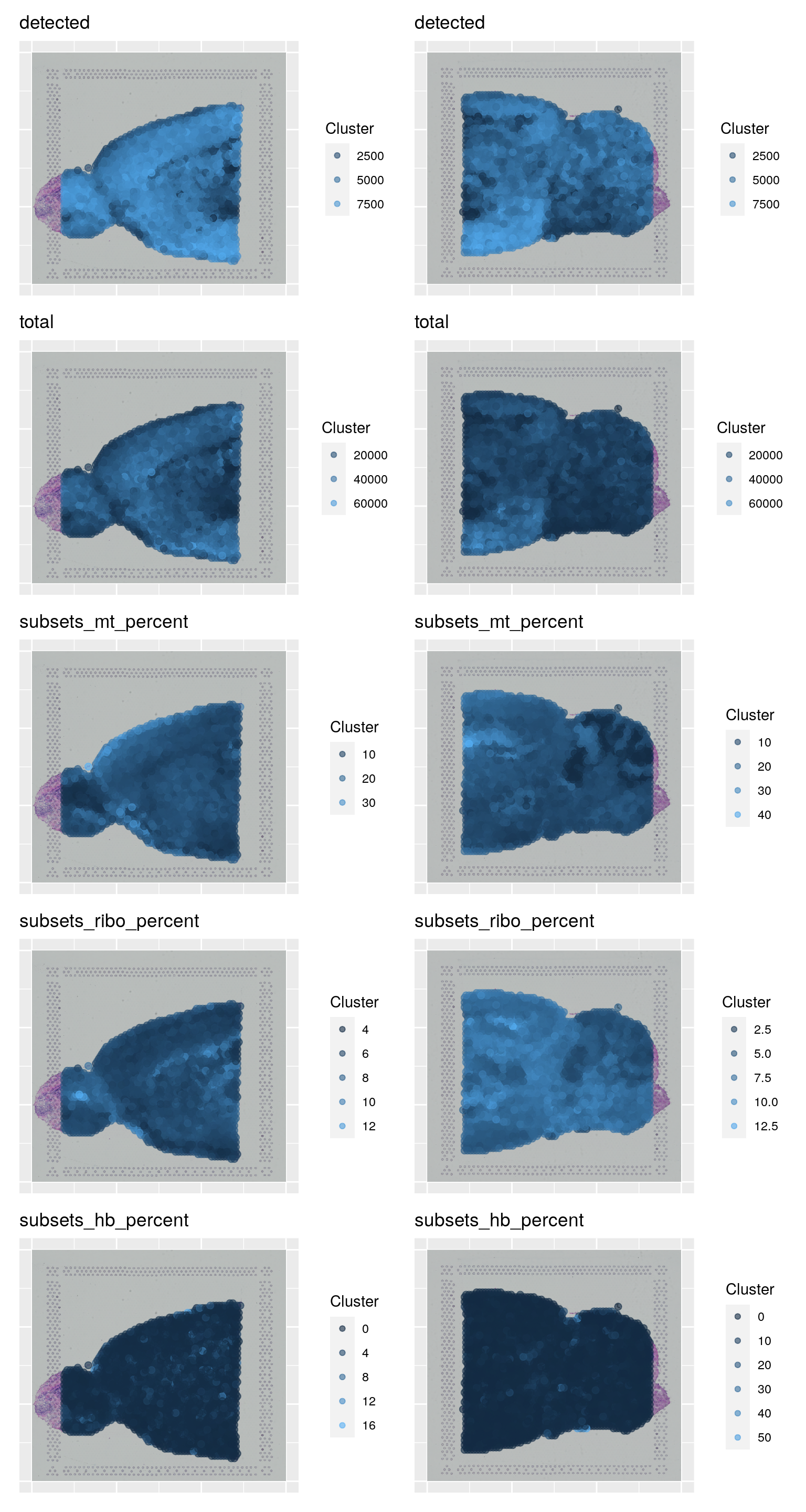
As you can see, the spots with low number of counts/features and high mitochondrial content are mainly towards the edges of the tissue. It is quite likely that these regions are damaged tissue. You may also see regions within a tissue with low quality if you have tears or folds in your section.
But remember, for some tissue types, the amount of genes expressed and proportion mitochondria may also be a biological features, so bear in mind what tissue you are working on and what these features mean.
2.1 Filter spots
Select all spots with less than 25% mitocondrial reads, less than 20% hb-reads and 500 detected genes. You must judge for yourself based on your knowledge of the tissue what are appropriate filtering criteria for your dataset.
sce <- sce[, sce$detected > 500 &
    sce$subsets_mt_percent < 25 &
    sce$subsets_hb_percent < 20]
dim(sce)
[1] 32053 5804And replot onto tissue section:
samples <- c("Anterior", "Posterior")
to_plot <- c("detected", "total", "subsets_mt_percent", "subsets_mt_percent", "subsets_hb_percent")

plist <- list()
n <- 1
for (j in to_plot) {
    for (i in samples) {
        temp <- sce[, sce$Sample == i]
        temp@metadata <- temp@metadata[[i]]
        plist[[n]] <- spanielPlot(
            object = temp,
            plotType = "Cluster",
            clusterRes = j, customTitle = j,
            techType = "Visium",
            ptSizeMax = 1, ptSizeMin = .1
        )
        n <- n + 1
    }
}

wrap_plots(plist, ncol = 2)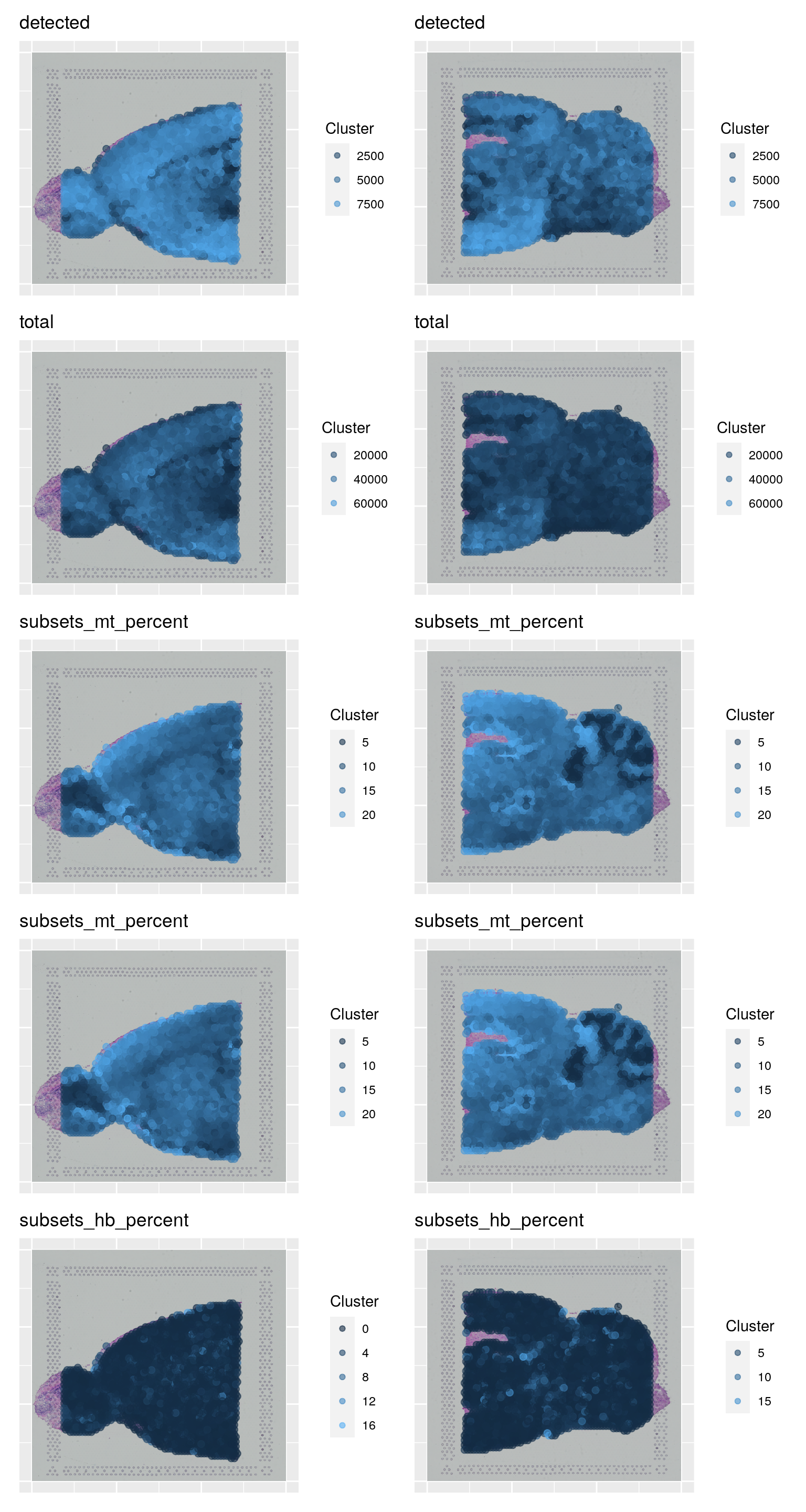
2.2 Top expressed genes
As for scRNA-seq data, we will look at what the top expressed genes are.
C <- counts(sce)
C@x <- C@x / rep.int(colSums(C), diff(C@p))
most_expressed <- order(Matrix::rowSums(C), decreasing = T)[20:1]
boxplot(as.matrix(t(C[most_expressed, ])), cex = .1, las = 1, xlab = "% total count per cell", col = scales::hue_pal()(20)[20:1], horizontal = TRUE)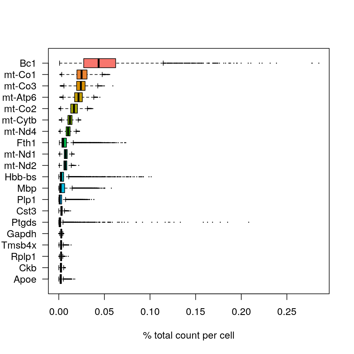
rm(C)As you can see, the mitochondrial genes are among the top expressed genes. Also the lncRNA gene Bc1 (brain cytoplasmic RNA 1). Also one hemoglobin gene.
2.3 Filter genes
We will remove the Bc1 gene, hemoglobin genes (blood contamination) and the mitochondrial genes.
dim(sce)[1] 32053 5804# Filter Bl1
sce <- sce[!grepl("Bc1", rownames(sce)), ]
# Filter Mitocondrial
sce <- sce[!grepl("^mt-", rownames(sce)), ]
# Filter Hemoglobin gene (optional if that is a problem on your data)
sce <- sce[!grepl("^Hb.*-", rownames(sce)), ]
dim(sce)[1] 32031 58043 Analysis
We will proceed with the data in a very similar manner to scRNA-seq data.
sce <- computeSumFactors(sce, sizes = c(20, 40, 60, 80))
sce <- logNormCounts(sce)
Now we can plot gene expression of individual genes, the gene Hpca is a strong hippocampal marker and Ttr is a marker of the choroid plexus.
samples <- c("Anterior", "Posterior")
to_plot <- c("Hpca", "Ttr")

plist <- list()
n <- 1
for (j in to_plot) {
    for (i in samples) {
        temp <- sce[, sce$Sample == i]
        temp@metadata <- temp@metadata[[i]]
        plist[[n]] <- spanielPlot(
            object = temp,
            plotType = "Gene",
            gene = j,
            customTitle = j,
            techType = "Visium",
            ptSizeMax = 1, ptSizeMin = .1
        )
        n <- n + 1
    }
}

wrap_plots(plist, ncol = 2)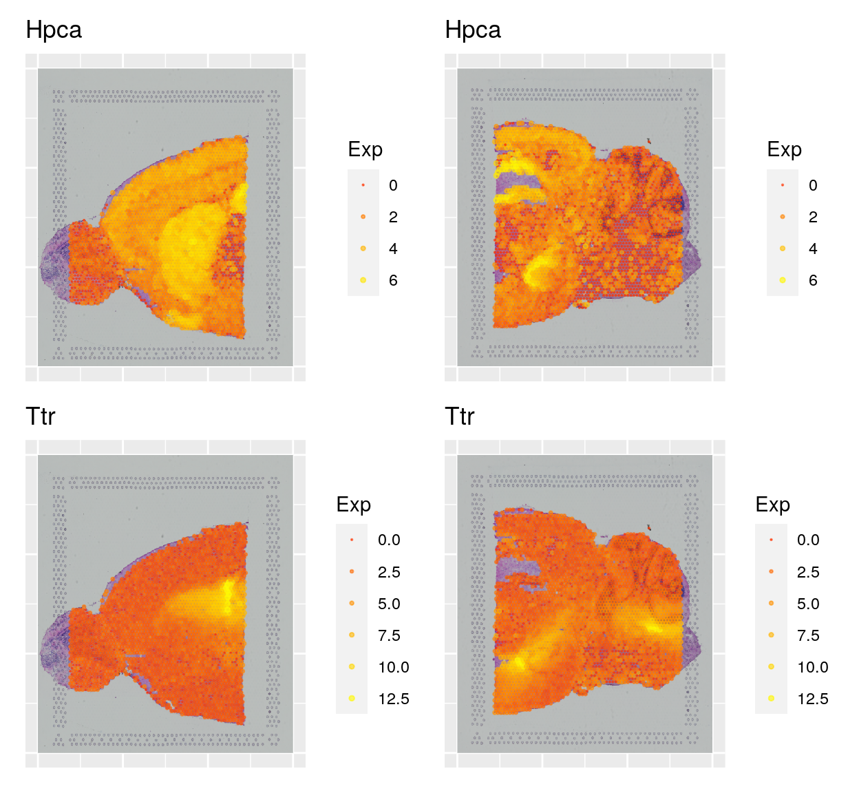
3.1 Dimensionality reduction and clustering
We can then now run dimensionality reduction and clustering using the same workflow as we use for scRNA-seq analysis.
But make sure you run it on the SCT assay.
var.out <- modelGeneVar(sce, method = "loess")
hvgs <- getTopHVGs(var.out, n = 2000)
sce <- runPCA(sce,
    exprs_values = "logcounts",
    subset_row = hvgs,
    ncomponents = 50,
    ntop = 100,
    scale = T
)
g <- buildSNNGraph(sce, k = 5, use.dimred = "PCA")
sce$louvain_SNNk5 <- factor(igraph::cluster_louvain(g)$membership)
sce <- runUMAP(sce,
    dimred = "PCA", n_dimred = 50, ncomponents = 2, min_dist = 0.1, spread = .3,
    metric = "correlation", name = "UMAP_on_PCA"
)
We can then plot clusters onto umap or onto the tissue section.
samples <- c("Anterior", "Posterior")
to_plot <- c("louvain_SNNk5")

plist <- list()
n <- 1
for (j in to_plot) {
    for (i in samples) {
        temp <- sce[, sce$Sample == i]
        temp@metadata <- temp@metadata[[i]]
        plist[[n]] <- spanielPlot(
            object = temp,
            plotType = "Cluster", clusterRes = j,
            customTitle = j,
            techType = "Visium",
            ptSizeMax = 1, ptSizeMin = .1
        )
        n <- n + 1
    }
}

plist[[3]] <- plotReducedDim(sce, dimred = "UMAP_on_PCA", colour_by = "louvain_SNNk5")
plist[[4]] <- plotReducedDim(sce, dimred = "UMAP_on_PCA", colour_by = "Sample")

wrap_plots(plist, ncol = 2)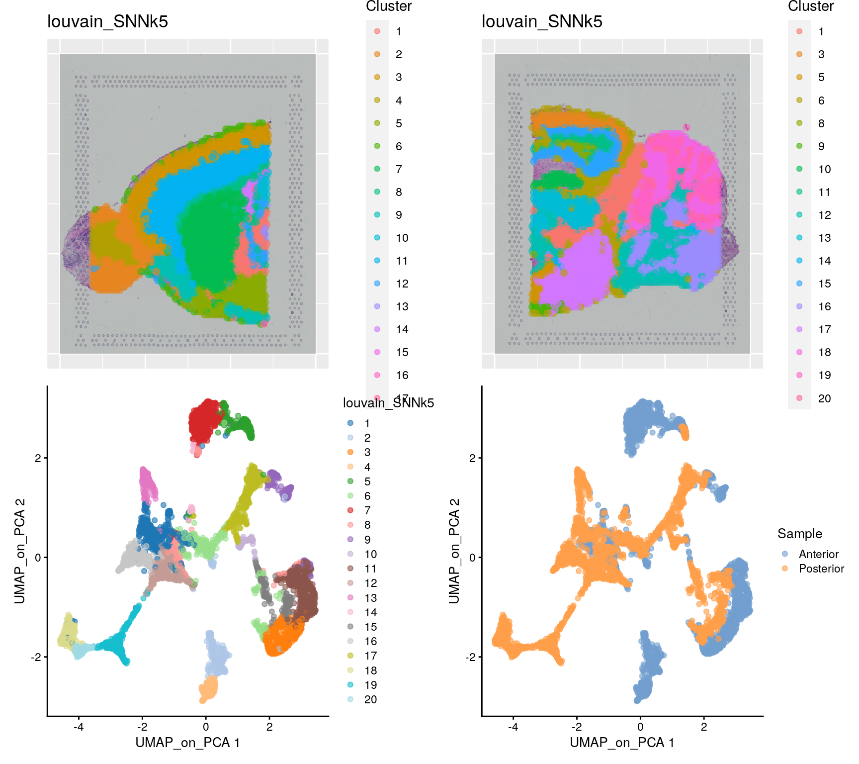
3.2 Integration
Quite often, there are strong batch effects between different ST sections, so it may be a good idea to integrate the data across sections.
We will do a similar integration as in the Data Integration lab.
mnn_out <- batchelor::fastMNN(sce, subset.row = hvgs, batch = factor(sce$Sample), k = 20, d = 50)

reducedDim(sce, "MNN") <- reducedDim(mnn_out, "corrected")
rm(mnn_out)
gc()
used (Mb) gc trigger (Mb) max used (Mb)
Ncells 10071516 537.9 14512824 775.1 14512824 775.1
Vcells 191851637 1463.8 373719786 2851.3 311584088 2377.2Then we run dimensionality reduction and clustering as before.
g <- buildSNNGraph(sce, k = 5, use.dimred = "MNN")
sce$louvain_SNNk5 <- factor(igraph::cluster_louvain(g)$membership)
sce <- runUMAP(sce,
    dimred = "MNN", n_dimred = 50, ncomponents = 2, min_dist = 0.1, spread = .3,
    metric = "correlation", name = "UMAP_on_MNN"
)
samples <- c("Anterior", "Posterior")
to_plot <- c("louvain_SNNk5")
plist <- list()
n <- 1
for (j in to_plot) {
for (i in samples) {
temp <- sce[, sce$Sample == i]
temp@metadata <- temp@metadata[[i]]
plist[[n]] <- spanielPlot(
object = temp,
plotType = "Cluster", clusterRes = j,
customTitle = j,
techType = "Visium",
ptSizeMax = 1, ptSizeMin = .1
)
n <- n + 1
}
}
plist[[3]] <- plotReducedDim(sce, dimred = "UMAP_on_MNN", colour_by = "louvain_SNNk5")
plist[[4]] <- plotReducedDim(sce, dimred = "UMAP_on_MNN", colour_by = "Sample")
wrap_plots(plist, ncol = 2)
Discuss
Do you see any differences between the integrated and non-integrated clustering? Judge for yourself, which of the clusterings do you think looks best? As a reference, you can compare to brain regions in the Allen brain atlas.
3.3 Spatially Variable Features
There are two main workflows to identify molecular features that correlate with spatial location within a tissue. The first is to perform differential expression based on spatially distinct clusters, the other is to find features that have spatial patterning without taking clusters or spatial annotation into account. First, we will do differential expression between clusters just as we did for the scRNAseq data before.
# differential expression between cluster 4 and cluster 6
cell_selection <- sce[, sce$louvain_SNNk5 %in% c(4, 6)]
cell_selection$louvain_SNNk5 <- factor(cell_selection$louvain_SNNk5)

markers_genes <- scran::findMarkers(
    x = cell_selection,
    groups = cell_selection$louvain_SNNk5,
    lfc = .25,
    pval.type = "all",
    direction = "up"
)

# List of dataFrames with the results for each cluster
top5_cell_selection <- lapply(names(markers_genes), function(x) {
    temp <- markers_genes[[x]][1:5, 1:2]
    temp$gene <- rownames(markers_genes[[x]])[1:5]
    temp$cluster <- x
    return(temp)
})
top5_cell_selection <- as_tibble(do.call(rbind, top5_cell_selection))
top5_cell_selection
# plot top markers
samples <- c("Anterior", "Posterior")
to_plot <- top5_cell_selection$gene[1:5]
plist <- list()
n <- 1
for (j in to_plot) {
for (i in samples) {
temp <- sce[, sce$Sample == i]
temp@metadata <- temp@metadata[[i]]
plist[[n]] <- spanielPlot(
object = temp,
plotType = "Gene",
gene = j,
customTitle = j,
techType = "Visium",
ptSizeMax = 1, ptSizeMin = .1
)
n <- n + 1
}
}
wrap_plots(plist, ncol = 2)
4 Single cell data
We can use a scRNA-seq dataset as a reference to predict the proportion of different celltypes in the Visium spots. Keep in mind that it is important to have a reference that contains all the celltypes you expect to find in your spots. Ideally it should be a scRNA-seq reference from the exact same tissue. We will use a reference scRNA-seq dataset of ~14,000 adult mouse cortical cell taxonomy from the Allen Institute, generated with the SMART-Seq2 protocol.
First dowload the seurat data:
path_file <- "data/spatial/visium/allen_cortex.rds"
if (!file.exists(path_file)) download.file(url = file.path(path_data, "spatial/visium/allen_cortex.rds"), destfile = path_file)
For speed, and for a more fair comparison of the celltypes, we will subsample all celltypes to a maximum of 200 cells per class (subclass).
ar <- readRDS(path_file)
ar_sce <- Seurat::as.SingleCellExperiment(ar)
rm(ar)
gc()
used (Mb) gc trigger (Mb) max used (Mb)
Ncells 10176203 543.5 18553912 990.9 18553912 990.9
Vcells 577996690 4409.8 833683239 6360.5 578399539 4412.9# check number of cells per subclass
ar_sce$subclass <- sub("/", "_", sub(" ", "_", ar_sce$subclass))
table(ar_sce$subclass)
     Astro         CR       Endo    L2_3_IT         L4      L5_IT      L5_PT
       368          7         94        982       1401        880        544
     L6_CT      L6_IT        L6b      Lamp5 Macrophage      Meis2         NP
       960       1872        358       1122         51         45        362
     Oligo       Peri      Pvalb   Serpinf1        SMC       Sncg        Sst
        91         32       1337         27         55        125       1741
       Vip       VLMC
      1728         67
# select 20 cells per subclass, fist set subclass as active.ident
subset_cells <- lapply(unique(ar_sce$subclass), function(x) {
if (sum(ar_sce$subclass == x) > 20) {
temp <- sample(colnames(ar_sce)[ar_sce$subclass == x], size = 20)
} else {
temp <- colnames(ar_sce)[ar_sce$subclass == x]
}
})
ar_sce <- ar_sce[, unlist(subset_cells)]
# check again number of cells per subclass
table(ar_sce$subclass)
     Astro         CR       Endo    L2_3_IT         L4      L5_IT      L5_PT
        20          7         20         20         20         20         20
     L6_CT      L6_IT        L6b      Lamp5 Macrophage      Meis2         NP
        20         20         20         20         20         20         20
     Oligo       Peri      Pvalb   Serpinf1        SMC       Sncg        Sst
        20         20         20         20         20         20         20
       Vip       VLMC
        20         20
Then run normalization and dimensionality reduction.
ar_sce <- computeSumFactors(ar_sce, sizes = c(20, 40, 60, 80))
ar_sce <- logNormCounts(ar_sce)
allen.var.out <- modelGeneVar(ar_sce, method = "loess")
allen.hvgs <- getTopHVGs(allen.var.out, n = 2000)
5 Subset ST for cortex
Since the scRNAseq dataset was generated from the mouse cortex, we will subset the visium dataset in order to select mainly the spots part of the cortex. Note that the integration can also be performed on the whole brain slice, but it would give rise to false positive cell type assignments and therefore it should be interpreted with more care.
5.1 Integrate with scRNAseq
Here, will use SingleR for prediciting which cell types are present in the dataset. We can first select the anterior part as an example (to speed up predictions).
sce.anterior <- sce[, sce$Sample == "Anterior"]
sce.anterior@metadata <- sce.anterior@metadata[["Anterior"]]
Next, we select the highly variable genes that are present in both datasets.
# Find common highly variable genes
common_hvgs <- intersect(allen.hvgs, hvgs)
# Predict cell classes
pred.grun <- SingleR(
test = sce.anterior[common_hvgs, ],
ref = ar_sce[common_hvgs, ],
labels = ar_sce$subclass
)
# Transfer the classes to the SCE object
sce.anterior$cell_prediction <- pred.grun$labels
sce.anterior@colData <- cbind(
sce.anterior@colData,
as.data.frame.matrix(table(list(1:ncol(sce.anterior), sce.anterior$cell_prediction)))
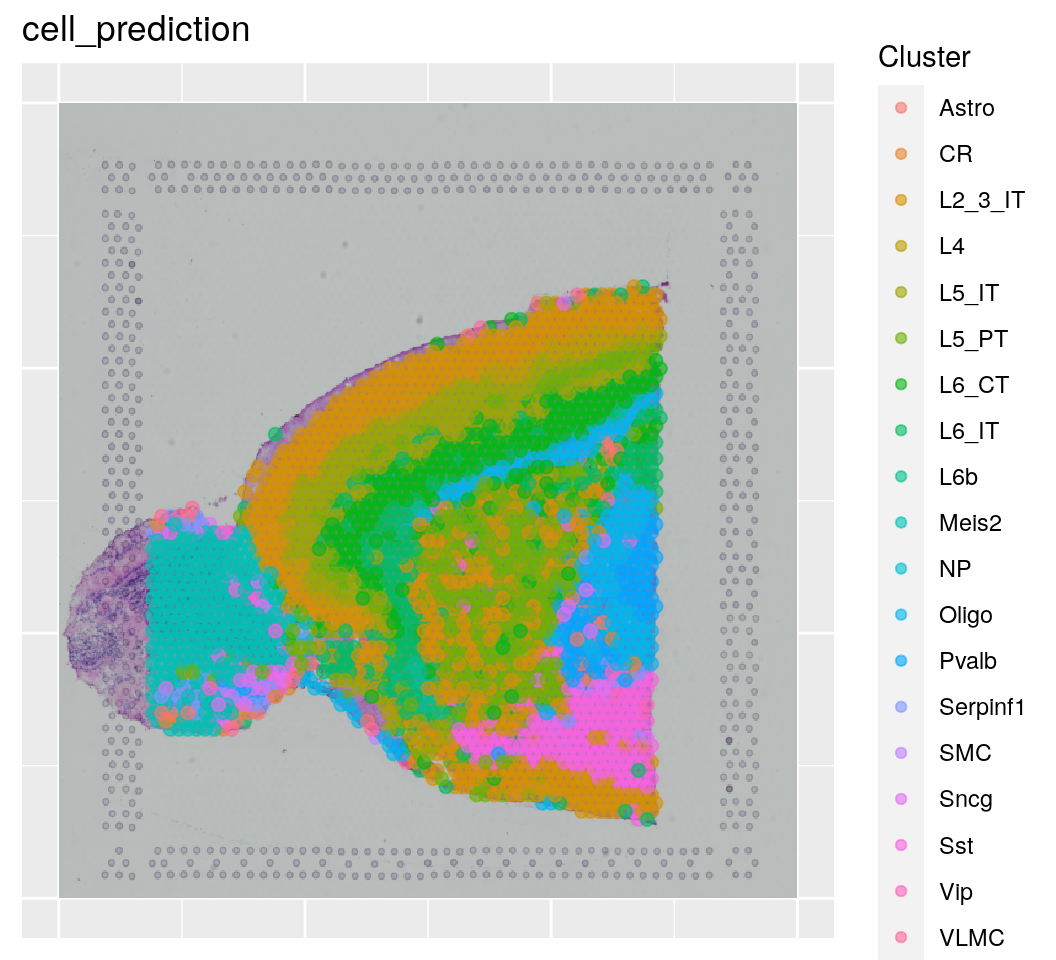
)Then we can plot the predicted cell populations back to tissue.
# Plot cell predictions
spanielPlot(
    object = sce.anterior,
    plotType = "Cluster",
    clusterRes = "cell_prediction",
    customTitle = "cell_prediction",
    techType = "Visium",
    ptSizeMax = 1, ptSizeMin = .1
)
plist <- list()
n <- 1
for (i in c("L2_3_IT", "L4", "L5_IT", "L6_IT")) {
    plist[[n]] <- spanielPlot(
        object = sce.anterior,
        plotType = "Cluster",
        clusterRes = i,
        customTitle = i,
        techType = "Visium", ptSize = .3,
        ptSizeMax = 1, ptSizeMin = .1
    )
    n <- n + 1
}
wrap_plots(plist, ncol = 2)
Keep in mind, that the scores are “just” prediction scores, and do not correspond to proportion of cells that are of a certain celltype or similar. It mainly tell you that gene expression in a certain spot is hihgly similar/dissimilar to gene expression of a celltype. If we look at the scores, we see that some spots got really clear predictions by celltype, while others did not have high scores for any of the celltypes.
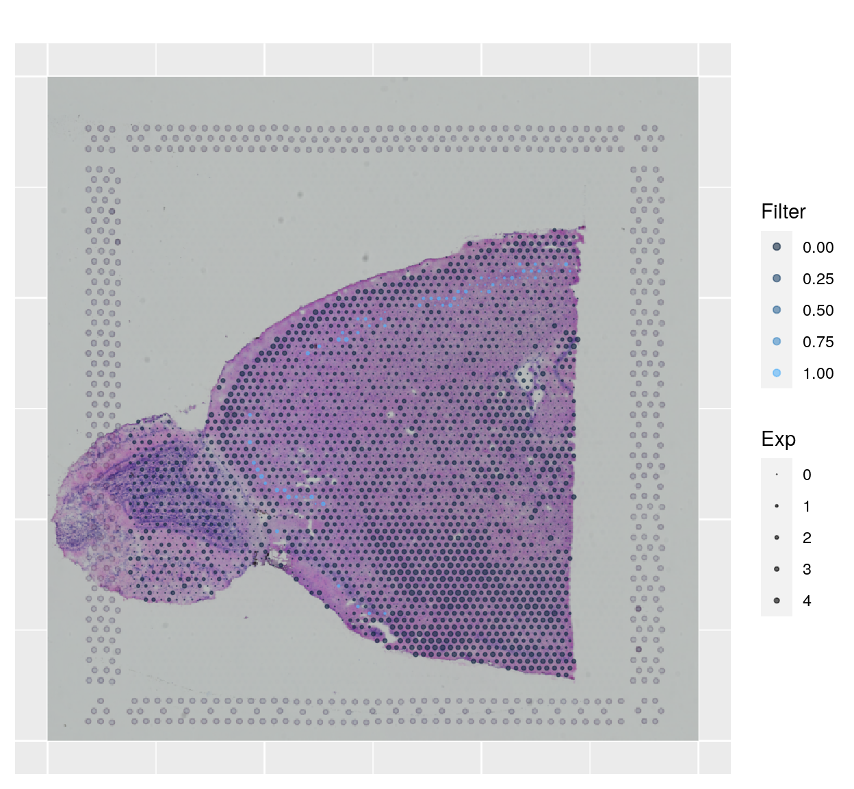
We can also plot the gene expression and add filters together, too:
spanielPlot(
    object = sce.anterior,
    plotType = "Gene",
    gene = "Wfs1",
    showFilter = sce.anterior$L4,
    customTitle = "",
    techType = "Visium",
    ptSize = 0, ptSizeMin = -.3, ptSizeMax = 1
)
6 Session info
Click here
sessionInfo()R version 4.3.0 (2023-04-21)
Platform: x86_64-pc-linux-gnu (64-bit)
Running under: Ubuntu 22.04.3 LTS
Matrix products: default
BLAS: /usr/lib/x86_64-linux-gnu/openblas-pthread/libblas.so.3
LAPACK: /usr/lib/x86_64-linux-gnu/openblas-pthread/libopenblasp-r0.3.20.so; LAPACK version 3.10.0
locale:
[1] LC_CTYPE=en_US.UTF-8 LC_NUMERIC=C
[3] LC_TIME=en_US.UTF-8 LC_COLLATE=en_US.UTF-8
[5] LC_MONETARY=en_US.UTF-8 LC_MESSAGES=en_US.UTF-8
[7] LC_PAPER=en_US.UTF-8 LC_NAME=C
[9] LC_ADDRESS=C LC_TELEPHONE=C
[11] LC_MEASUREMENT=en_US.UTF-8 LC_IDENTIFICATION=C
time zone: Etc/UTC
tzcode source: system (glibc)
attached base packages:
[1] stats4 stats graphics grDevices utils datasets methods
[8] base
other attached packages:
[1] patchwork_1.1.2 scater_1.30.1
[3] ggplot2_3.4.2 SingleR_2.4.1
[5] scran_1.30.0 scuttle_1.12.0
[7] dplyr_1.1.2 Matrix_1.5-4
[9] SingleCellExperiment_1.24.0 SummarizedExperiment_1.32.0
[11] Biobase_2.62.0 GenomicRanges_1.54.1
[13] GenomeInfoDb_1.38.5 IRanges_2.36.0
[15] S4Vectors_0.40.2 BiocGenerics_0.48.1
[17] MatrixGenerics_1.14.0 matrixStats_1.0.0
[19] Spaniel_1.16.0
loaded via a namespace (and not attached):
[1] RcppAnnoy_0.0.20 batchelor_1.18.1
[3] splines_4.3.0 later_1.3.1
[5] bitops_1.0-7 R.oo_1.25.0
[7] tibble_3.2.1 polyclip_1.10-4
[9] lifecycle_1.0.3 edgeR_4.0.7
[11] globals_0.16.2 lattice_0.21-8
[13] MASS_7.3-58.4 magrittr_2.0.3
[15] limma_3.58.1 plotly_4.10.2
[17] rmarkdown_2.22 yaml_2.3.7
[19] metapod_1.10.1 httpuv_1.6.11
[21] Seurat_4.3.0 sctransform_0.3.5
[23] sp_1.6-1 spatstat.sparse_3.0-1
[25] reticulate_1.30 cowplot_1.1.1
[27] pbapply_1.7-0 RColorBrewer_1.1-3
[29] ResidualMatrix_1.12.0 abind_1.4-5
[31] zlibbioc_1.48.0 Rtsne_0.16
[33] R.utils_2.12.2 purrr_1.0.1
[35] RCurl_1.98-1.12 GenomeInfoDbData_1.2.11
[37] ggrepel_0.9.3 irlba_2.3.5.1
[39] listenv_0.9.0 spatstat.utils_3.0-3
[41] goftest_1.2-3 spatstat.random_3.1-5
[43] dqrng_0.3.0 fitdistrplus_1.1-11
[45] parallelly_1.36.0 DelayedMatrixStats_1.24.0
[47] DropletUtils_1.22.0 leiden_0.4.3
[49] codetools_0.2-19 DelayedArray_0.28.0
[51] tidyselect_1.2.0 farver_2.1.1
[53] viridis_0.6.3 ScaledMatrix_1.10.0
[55] spatstat.explore_3.2-1 jsonlite_1.8.5
[57] BiocNeighbors_1.20.2 ellipsis_0.3.2
[59] progressr_0.13.0 ggridges_0.5.4
[61] survival_3.5-5 tools_4.3.0
[63] ica_1.0-3 Rcpp_1.0.10
[65] glue_1.6.2 gridExtra_2.3
[67] SparseArray_1.2.3 xfun_0.39
[69] HDF5Array_1.30.0 withr_2.5.0
[71] fastmap_1.1.1 rhdf5filters_1.14.1
[73] bluster_1.12.0 fansi_1.0.4
[75] digest_0.6.31 rsvd_1.0.5
[77] R6_2.5.1 mime_0.12
[79] colorspace_2.1-0 scattermore_1.2
[81] tensor_1.5 spatstat.data_3.0-1
[83] R.methodsS3_1.8.2 utf8_1.2.3
[85] tidyr_1.3.0 generics_0.1.3
[87] data.table_1.14.8 httr_1.4.6
[89] htmlwidgets_1.6.2 S4Arrays_1.2.0
[91] uwot_0.1.14 pkgconfig_2.0.3
[93] gtable_0.3.3 lmtest_0.9-40
[95] XVector_0.42.0 htmltools_0.5.5
[97] SeuratObject_4.1.3 scales_1.2.1
[99] png_0.1-8 knitr_1.43
[101] rstudioapi_0.14 reshape2_1.4.4
[103] nlme_3.1-162 rhdf5_2.46.1
[105] zoo_1.8-12 stringr_1.5.0
[107] KernSmooth_2.23-20 parallel_4.3.0
[109] miniUI_0.1.1.1 vipor_0.4.5
[111] pillar_1.9.0 grid_4.3.0
[113] vctrs_0.6.2 RANN_2.6.1
[115] promises_1.2.0.1 BiocSingular_1.18.0
[117] beachmat_2.18.0 xtable_1.8-4
[119] cluster_2.1.4 beeswarm_0.4.0
[121] evaluate_0.21 cli_3.6.1
[123] locfit_1.5-9.8 compiler_4.3.0
[125] rlang_1.1.1 crayon_1.5.2
[127] future.apply_1.11.0 labeling_0.4.2
[129] plyr_1.8.8 ggbeeswarm_0.7.2
[131] stringi_1.7.12 viridisLite_0.4.2
[133] deldir_1.0-9 BiocParallel_1.36.0
[135] munsell_0.5.0 lazyeval_0.2.2
[137] spatstat.geom_3.2-1 sparseMatrixStats_1.14.0
[139] future_1.32.0 Rhdf5lib_1.24.1
[141] statmod_1.5.0 shiny_1.7.4
[143] ROCR_1.0-11 igraph_1.4.3