suppressPackageStartupMessages({
    library(scater)
    library(scran)
    # library(venn)
    library(patchwork)
    library(ggplot2)
    library(pheatmap)
    library(igraph)
    library(dplyr)
})
Note
Code chunks run R commands unless otherwise specified.
In this tutorial we will cover differential gene expression, which comprises an extensive range of topics and methods. In single cell, differential expresison can have multiple functionalities such as identifying marker genes for cell populations, as well as identifying differentially regulated genes across conditions (healthy vs control). We will also cover controlling batch effect in your test.
We can first load the data from the clustering session. Moreover, we can already decide which clustering resolution to use. First let’s define using the louvain clustering to identifying differentially expressed genes.
# download pre-computed data if missing or long compute
fetch_data <- TRUE

# url for source and intermediate data
path_data <- "https://nextcloud.dc.scilifelab.se/public.php/webdav"
curl_upass <- "-u zbC5fr2LbEZ9rSE:scRNAseq2025"

path_file <- "data/covid/results/bioc_covid_qc_dr_int_cl.rds"
if (!dir.exists(dirname(path_file))) dir.create(dirname(path_file), recursive = TRUE)
if (fetch_data && !file.exists(path_file)) download.file(url = file.path(path_data, "covid/results_bioc/bioc_covid_qc_dr_int_cl.rds"), destfile = path_file, method = "curl", extra = curl_upass)

sce <- readRDS(path_file)
print(reducedDims(sce))
List of length 17
names(17): PCA UMAP tSNE_on_PCA UMAP_on_PCA ... UMAP_on_Scanorama SNN harmony21 ?meta:dge_numbers
?meta:dge_numbers_1
However, findMarker in Scran is implemented so that the tests are run in a pariwise manner, e.g. each cluster is tested agains all the others individually. Then a combined p-value is calculated across all the tests using combineMarkers. So for this method, one large cluster will not influence the results in the same way as FindMarkers in Seurat or rank_genes_groups in Scanpy.
2 Cell marker genes
Let us first compute a ranking for the highly differential genes in each cluster. There are many different tests and parameters to be chosen that can be used to refine your results. When looking for marker genes, we want genes that are positively expressed in a cell type and possibly not expressed in others.
In the scran function findMarkers t-test, wilcoxon test and binomial test implemented.
# Compute differentiall expression
markers_genes <- scran::findMarkers(
    x = sce,
    groups = as.character(sce$leiden_k20),
    test.type = "wilcox",
    lfc = .5,
    pval.type = "all",
    direction = "up"
)

# List of dataFrames with the results for each cluster
markers_genes
List of length 12
names(12): 1 10 11 12 2 3 4 5 6 7 8 9# Visualizing the expression of one
head(markers_genes[["1"]])DataFrame with 6 rows and 14 columns
p.value FDR summary.AUC AUC.10 AUC.11 AUC.12
<numeric> <numeric> <numeric> <numeric> <numeric> <numeric>
PF4 3.37278e-18 6.35905e-14 0.935390 0.897980 0.932802 0.935390
PPBP 1.15151e-14 1.08553e-10 0.885631 0.830535 0.889347 0.885631
NRGN 1.28153e-13 8.05400e-10 0.869891 0.792515 0.877613 0.869891
OST4 1.69723e-09 7.99991e-06 0.799061 0.706455 0.880455 0.799061
GNG11 4.60120e-08 1.73502e-04 0.768977 0.744396 0.761918 0.768977
HIST1H2AC 1.01064e-03 1.00000e+00 0.654227 0.630455 0.655849 0.654227
AUC.2 AUC.3 AUC.4 AUC.5 AUC.6 AUC.7 AUC.8
<numeric> <numeric> <numeric> <numeric> <numeric> <numeric> <numeric>
PF4 0.930648 0.917763 0.931639 0.931273 0.919467 0.932478 0.925681
PPBP 0.881516 0.857537 0.882751 0.882185 0.865840 0.886964 0.860149
NRGN 0.873023 0.841010 0.874052 0.873096 0.848776 0.877458 0.852290
OST4 0.824765 0.818917 0.782093 0.791204 0.841604 0.827011 0.796163
GNG11 0.765071 0.753785 0.768578 0.765982 0.760749 0.768009 0.765285
HIST1H2AC 0.645704 0.644682 0.653331 0.652938 0.649382 0.653188 0.646287
AUC.9
<numeric>
PF4 0.925193
PPBP 0.874160
NRGN 0.858437
OST4 0.845740
GNG11 0.760696
HIST1H2AC 0.647491We can now select the top 25 overexpressed genes for plotting.
# Colect the top 25 genes for each cluster and put the into a single table
top25 <- lapply(names(markers_genes), function(x) {
temp <- markers_genes[[x]][1:25, 1:2]
temp$gene <- rownames(markers_genes[[x]])[1:25]
temp$cluster <- x
return(temp)
})
top25 <- as_tibble(do.call(rbind, top25))
top25$p.value[top25$p.value == 0] <- 1e-300
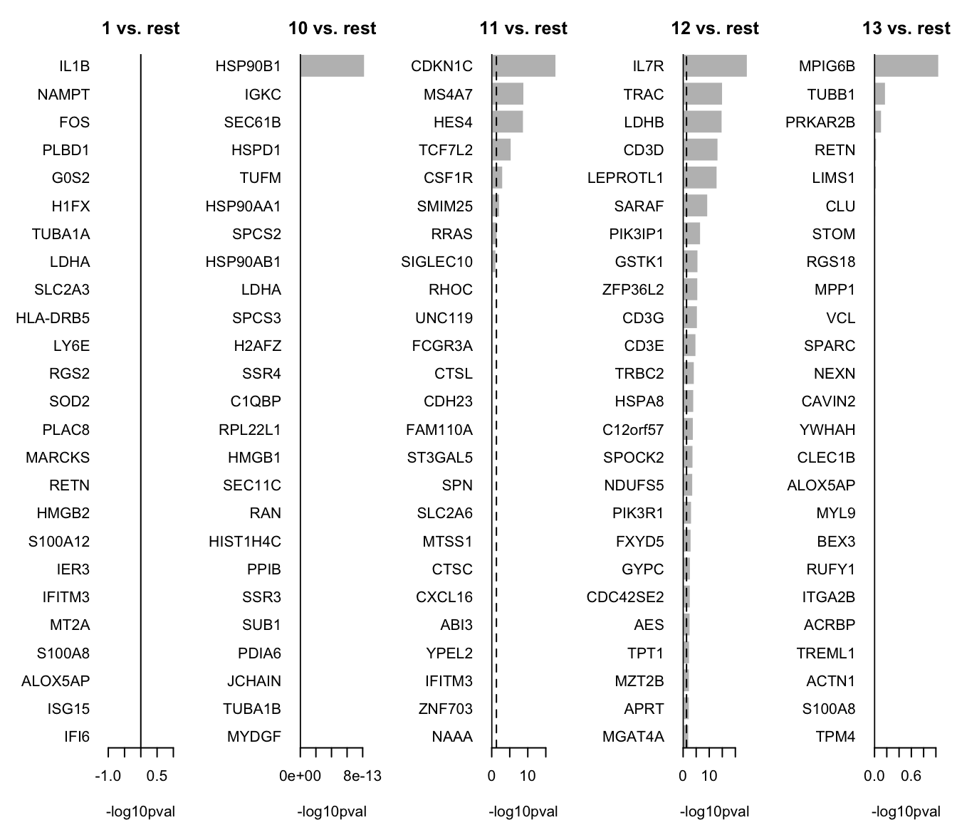
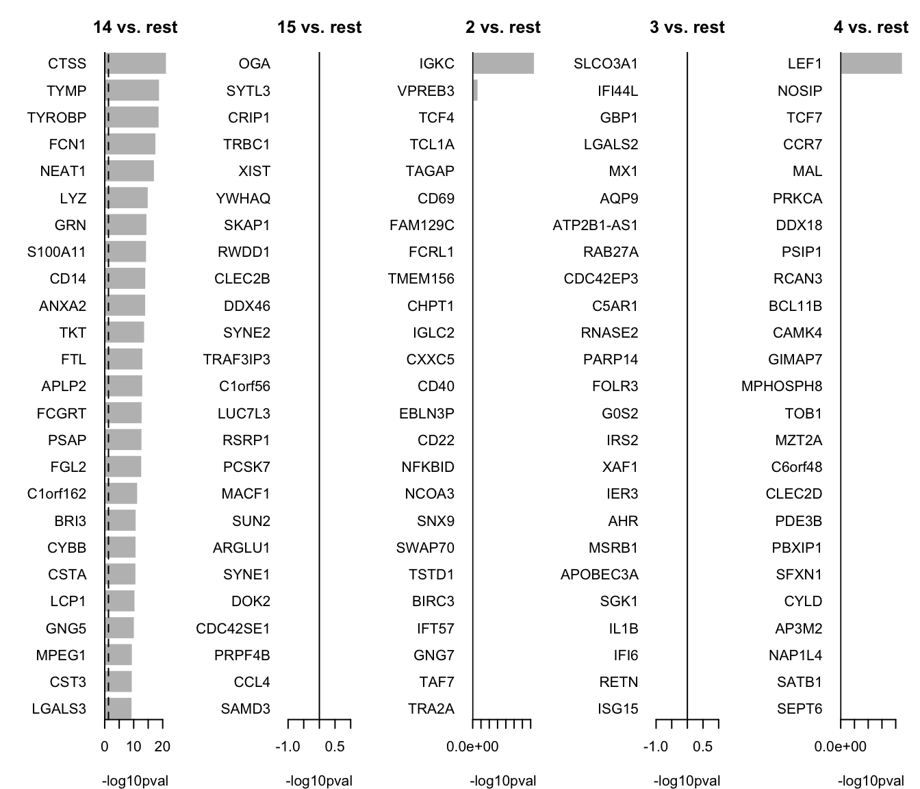
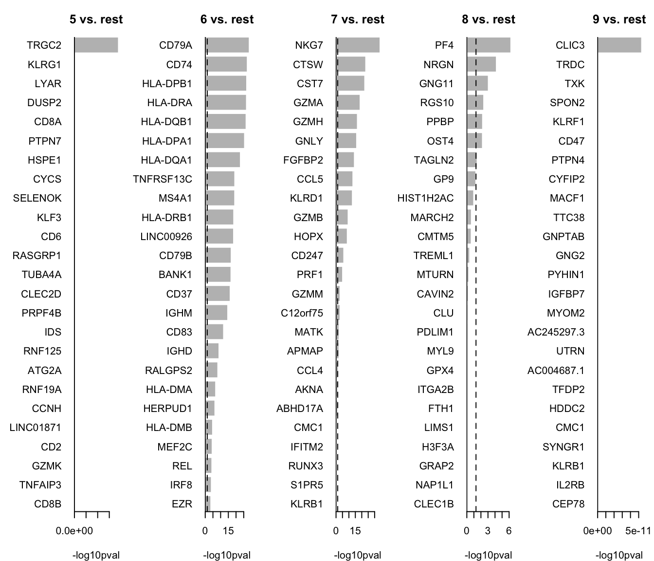
top25We can plot them as barplots per cluster.
par(mfrow = c(1, 5), mar = c(4, 6, 3, 1))
for (i in unique(top25$cluster)) {
    barplot(sort(setNames(-log10(top25$p.value), top25$gene)[top25$cluster == i], F),
        horiz = T, las = 1, main = paste0(i, " vs. rest"), border = "white", yaxs = "i", xlab = "-log10pval"
    )
    abline(v = c(0, -log10(0.05)), lty = c(1, 2))
}
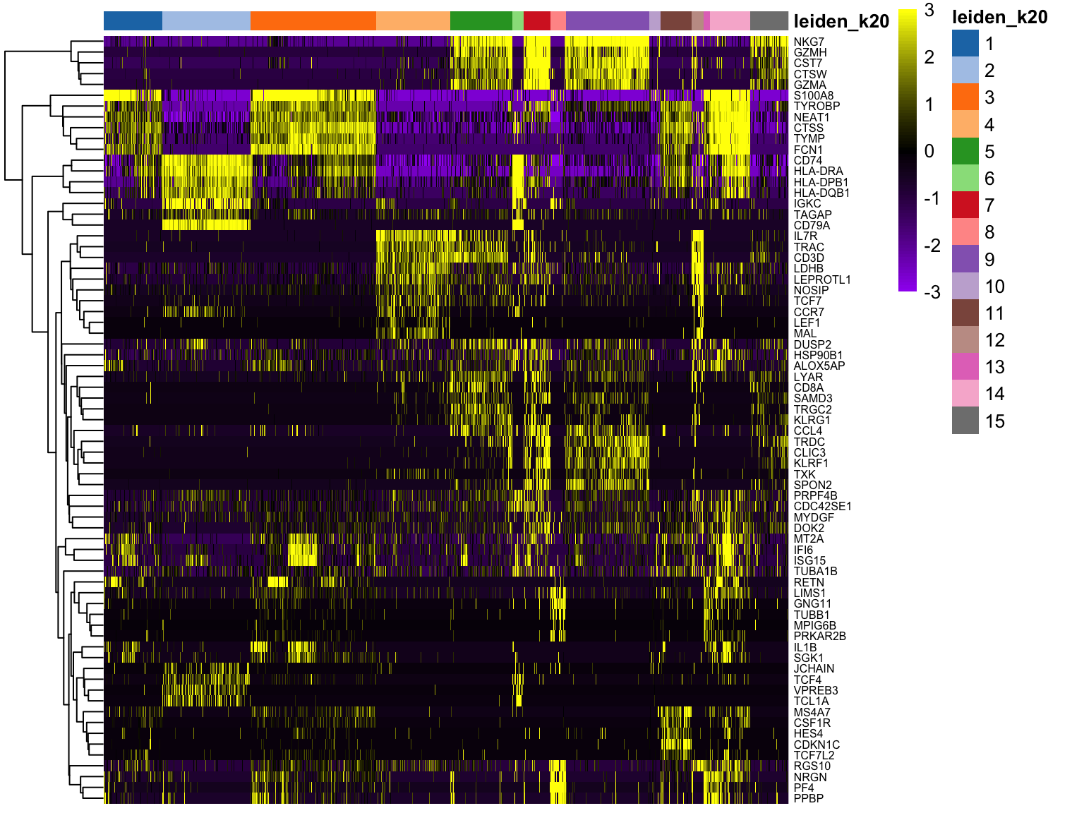
We can visualize them as a heatmap. Here we are selecting the top 5.
top25 %>%
    group_by(cluster) %>%
    slice_min(p.value, n = 5, with_ties = FALSE) -> top5


scater::plotHeatmap(sce[, order(sce$leiden_k20)],
    features = unique(top5$gene),
    center = T, zlim = c(-3, 3),
    colour_columns_by = "leiden_k20",
    show_colnames = F, cluster_cols = F,
    fontsize_row = 6,
    color = colorRampPalette(c("purple", "black", "yellow"))(90)
)
We can also plot a violin plot for each gene.
scater::plotExpression(sce, features = unique(top5$gene), x = "leiden_k20", ncol = 5, colour_by = "leiden_k20", scales = "free")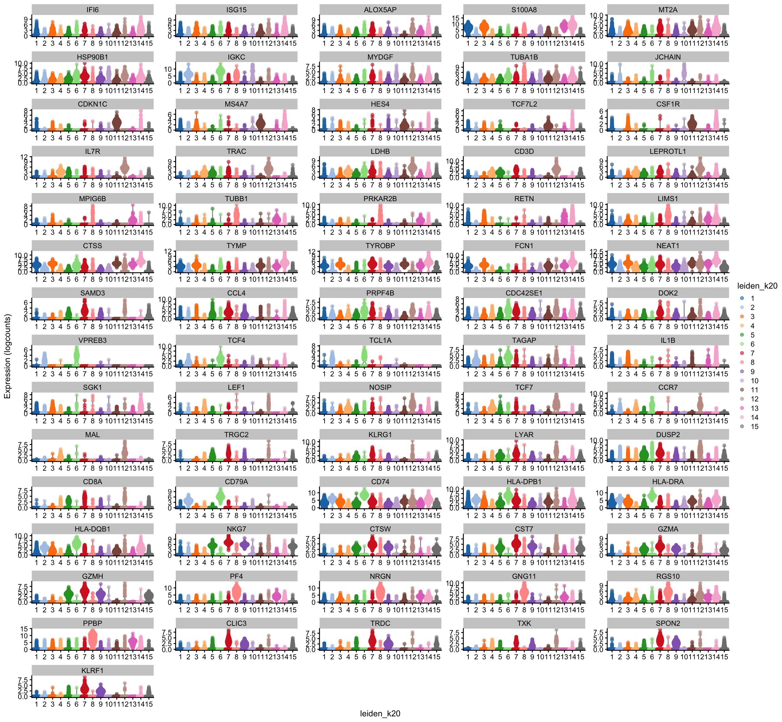
Another way is by representing the overall group expression and detection rates in a dot-plot.
plotDots(sce, features = unique(top5$gene), group="leiden_k20")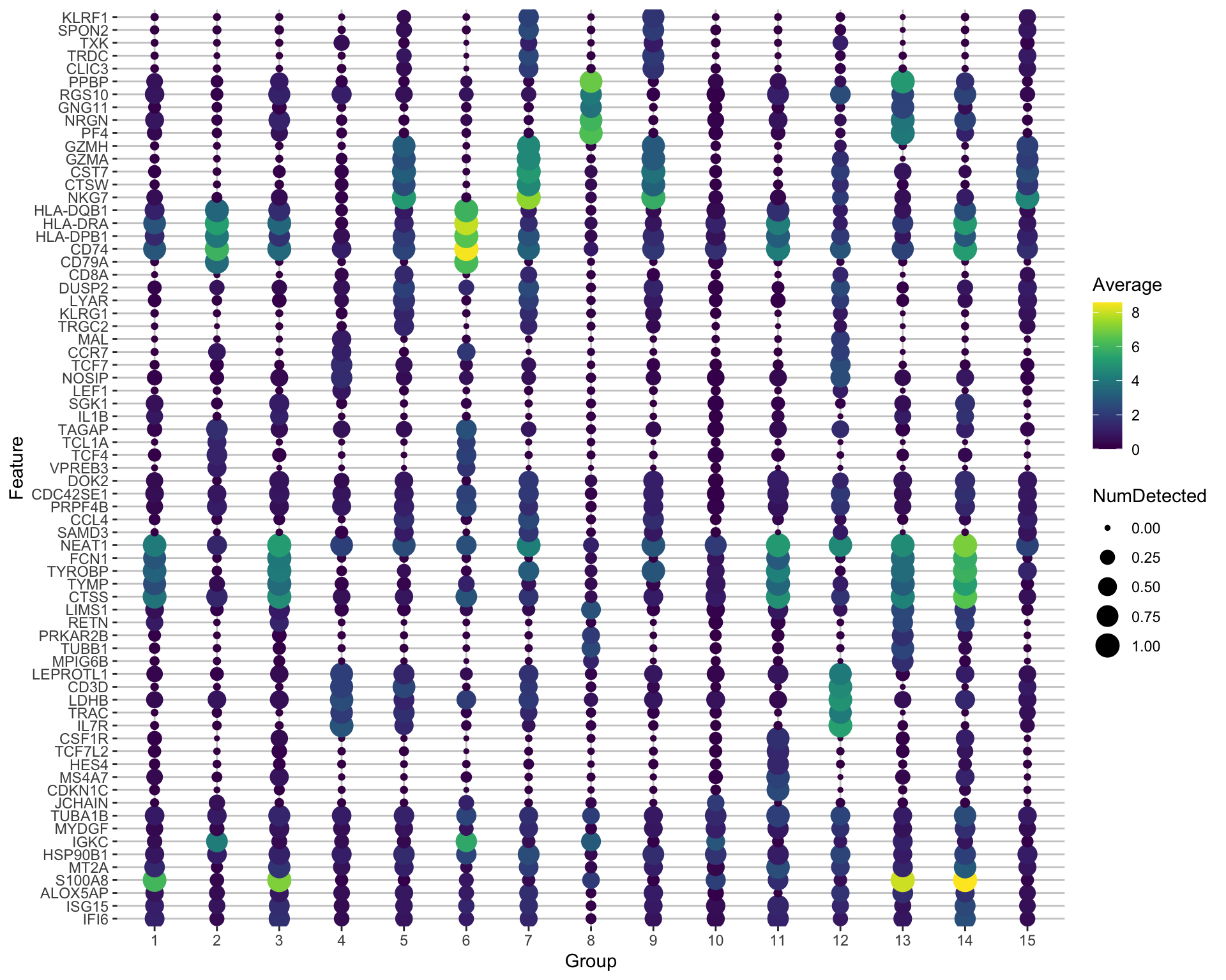
3 DGE across conditions
The second way of computing differential expression is to answer which genes are differentially expressed within a cluster. For example, in our case we have libraries comming from patients and controls and we would like to know which genes are influenced the most in a particular cell type. For this end, we will first subset our data for the desired cell cluster, then change the cell identities to the variable of comparison (which now in our case is the type, e.g. Covid/Ctrl).
# Filter cells from that cluster
cell_selection <- sce[, sce$leiden_k20 == 2]

# Compute differentiall expression
DGE_cell_selection <- findMarkers(
    x = cell_selection,
    groups = cell_selection@colData$type,
    lfc = .25,
    pval.type = "all",
    direction = "any"
)
top5_cell_selection <- lapply(names(DGE_cell_selection), function(x) {
    temp <- DGE_cell_selection[[x]][1:5, 1:2]
    temp$gene <- rownames(DGE_cell_selection[[x]])[1:5]
    temp$cluster <- x
    return(temp)
})
top5_cell_selection <- as_tibble(do.call(rbind, top5_cell_selection))
top5_cell_selection
We can now plot the expression across the type.
scater::plotExpression(cell_selection, features = unique(top5_cell_selection$gene), x = "type", ncol = 5, colour_by = "type")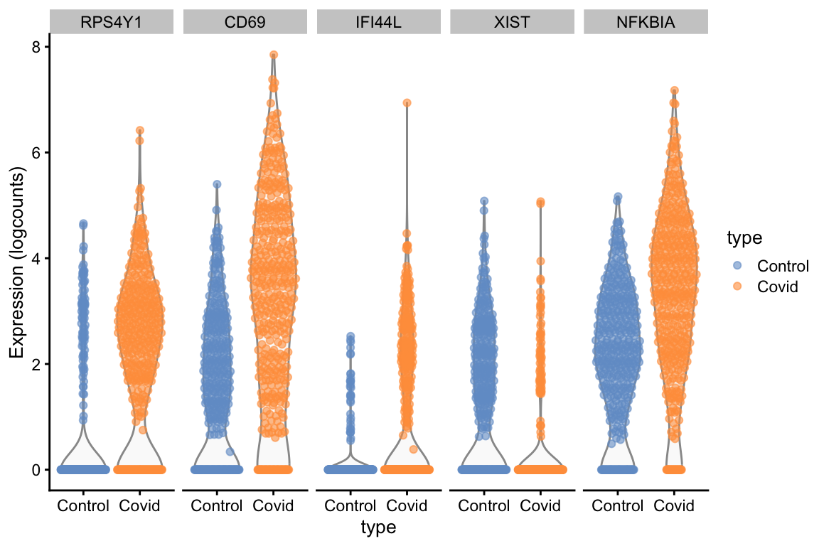
Or we can plot them as dotplots to see the expression in each individual sample.
plotDots(cell_selection, unique(top5_cell_selection$gene), group="sample")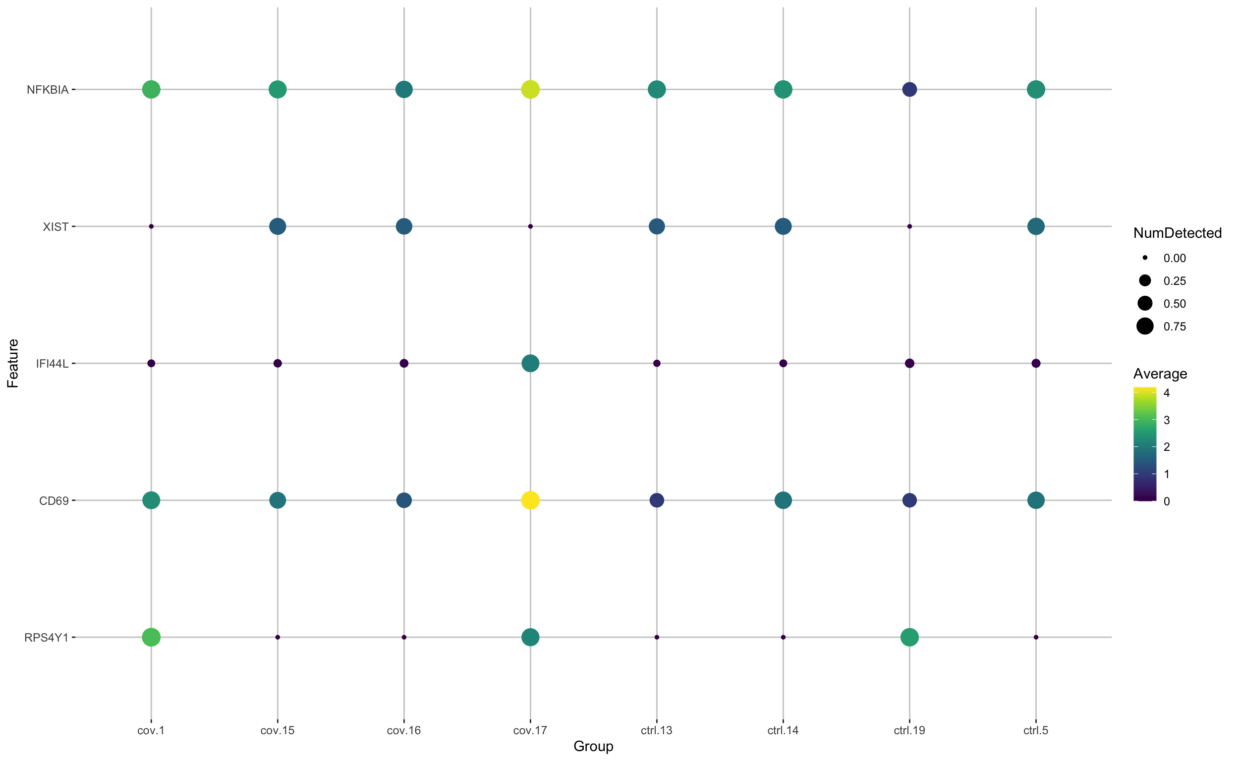
Clearly many of the top Covid genes are only high in the covid_17 sample, and not a general feature of covid patients. In this case using a method that can control for pseudreplication or pseudobulk methods would be appropriate. We have a more thorough discussion on this issue with sample batch effects in differential expression across conditions in the Seurat tutorial.
4 Gene Set Analysis (GSA)
4.1 Hypergeometric enrichment test
Having a defined list of differentially expressed genes, you can now look for their combined function using hypergeometric test.
# Load additional packages
library(enrichR)

# Check available databases to perform enrichment (then choose one)
enrichR::listEnrichrDbs()
# Perform enrichment
top_DGE <- DGE_cell_selection$Covid[(DGE_cell_selection$Covid$p.value < 0.01) & (abs(DGE_cell_selection$Covid[, grep("logFC.C", colnames(DGE_cell_selection$Covid))]) > 0.25), ]
enrich_results <- enrichr(
genes = rownames(top_DGE),
databases = "GO_Biological_Process_2017b"
)[[1]]Uploading data to Enrichr... Done.
Querying GO_Biological_Process_2017b... Done.
Parsing results... Done.Some databases of interest:
GO_Biological_Process_2017bKEGG_2019_HumanKEGG_2019_MouseWikiPathways_2019_HumanWikiPathways_2019_Mouse
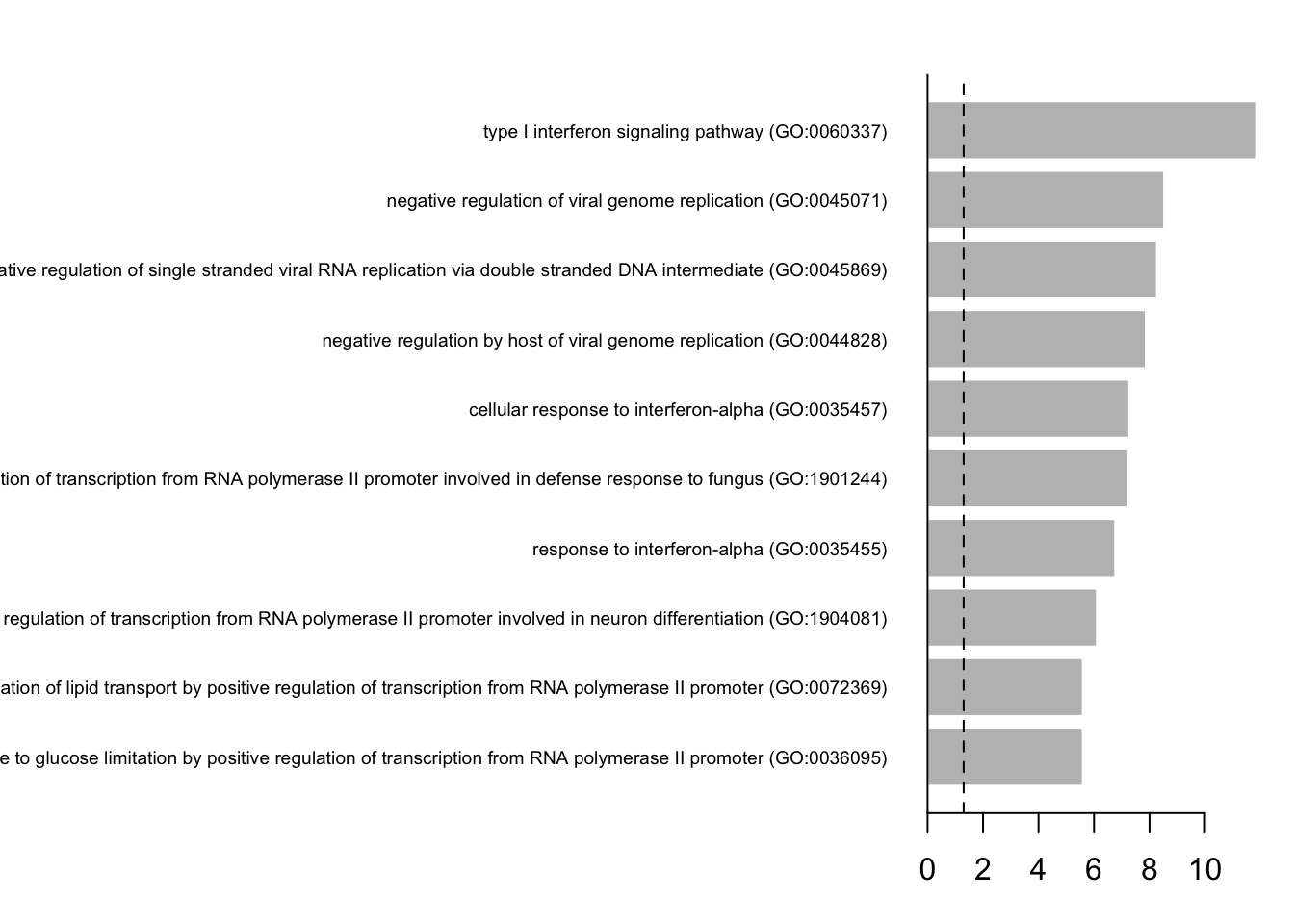
You visualize your results using a simple barplot, for example:
{
    par(mfrow = c(1, 1), mar = c(3, 25, 2, 1))
    barplot(
        height = -log10(enrich_results$P.value)[10:1],
        names.arg = enrich_results$Term[10:1],
        horiz = TRUE,
        las = 1,
        border = FALSE,
        cex.names = .6
    )
    abline(v = c(-log10(0.05)), lty = 2)
    abline(v = 0, lty = 1)
}
5 Gene Set Enrichment Analysis (GSEA)
Besides the enrichment using hypergeometric test, we can also perform gene set enrichment analysis (GSEA), which scores ranked genes list (usually based on fold changes) and computes permutation test to check if a particular gene set is more present in the Up-regulated genes, among the DOWN_regulated genes or not differentially regulated.
# Create a gene rank based on the gene expression fold change
gene_rank <- setNames(DGE_cell_selection$Covid[, grep("logFC.C", colnames(DGE_cell_selection$Covid))], casefold(rownames(DGE_cell_selection$Covid), upper = T))
Once our list of genes are sorted, we can proceed with the enrichment itself. We can use the package to get gene set from the Molecular Signature Database (MSigDB) and select KEGG pathways as an example.
library(msigdbr)

# Download gene sets
msigdbgmt <- msigdbr::msigdbr("Homo sapiens")
msigdbgmt <- as.data.frame(msigdbgmt)

# List available gene sets
unique(msigdbgmt$gs_subcat)
[1] "MIR:MIR_Legacy" "TFT:TFT_Legacy" "CGP" "TFT:GTRD"
[5] "" "VAX" "CP:BIOCARTA" "CGN"
[9] "GO:BP" "GO:CC" "IMMUNESIGDB" "GO:MF"
[13] "HPO" "CP:KEGG" "MIR:MIRDB" "CM"
[17] "CP" "CP:PID" "CP:REACTOME" "CP:WIKIPATHWAYS"# Subset which gene set you want to use.
msigdbgmt_subset <- msigdbgmt[msigdbgmt$gs_subcat == "CP:WIKIPATHWAYS", ]
gmt <- lapply(unique(msigdbgmt_subset$gs_name), function(x) {
msigdbgmt_subset[msigdbgmt_subset$gs_name == x, "gene_symbol"]
})
names(gmt) <- unique(paste0(msigdbgmt_subset$gs_name, "_", msigdbgmt_subset$gs_exact_source))Next, we will run GSEA. This will result in a table containing information for several pathways. We can then sort and filter those pathways to visualize only the top ones. You can select/filter them by either p-value or normalized enrichment score (NES).
library(fgsea)

# Perform enrichemnt analysis
fgseaRes <- fgsea(pathways = gmt, stats = gene_rank, minSize = 15, maxSize = 500, nperm = 10000)
fgseaRes <- fgseaRes[order(fgseaRes$NES, decreasing = T), ]

# Filter the results table to show only the top 10 UP or DOWN regulated processes (optional)
top10_UP <- fgseaRes$pathway[1:10]

# Nice summary table (shown as a plot)
plotGseaTable(gmt[top10_UP], gene_rank, fgseaRes, gseaParam = 0.5)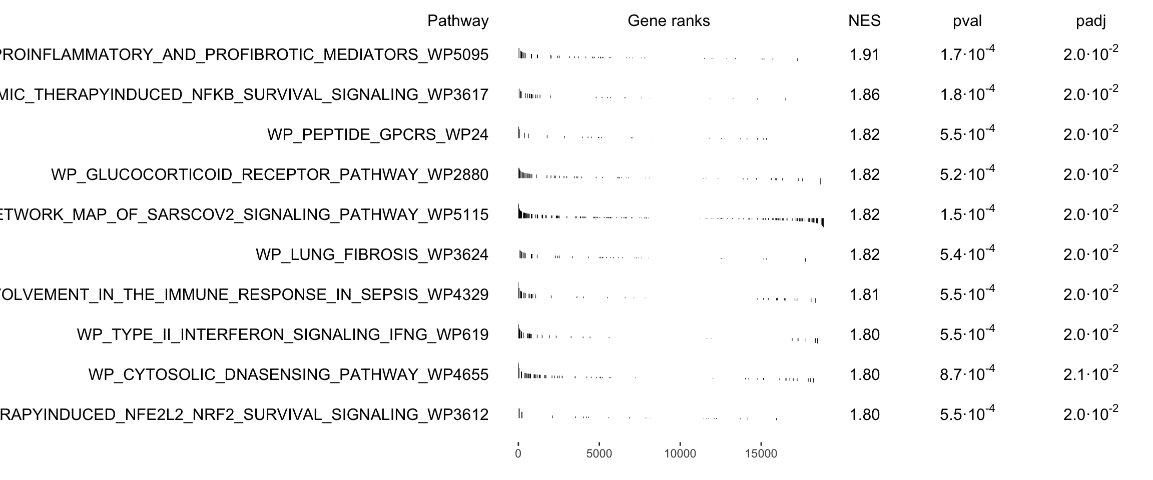
Discuss
Which KEGG pathways are upregulated in this cluster? Which KEGG pathways are dowregulated in this cluster? Change the pathway source to another gene set (e.g. CP:WIKIPATHWAYS or CP:REACTOME or CP:BIOCARTA or GO:BP) and check the if you get similar results?
Finally, let’s save the integrated data for further analysis.
saveRDS(sce, "data/covid/results/bioc_covid_qc_dr_int_cl_dge.rds")6 Session info
Click here
sessionInfo()R version 4.3.3 (2024-02-29)
Platform: x86_64-conda-linux-gnu (64-bit)
Running under: Ubuntu 20.04.6 LTS
Matrix products: default
BLAS/LAPACK: /usr/local/conda/envs/seurat/lib/libopenblasp-r0.3.28.so; LAPACK version 3.12.0
locale:
[1] LC_CTYPE=en_US.UTF-8 LC_NUMERIC=C
[3] LC_TIME=en_US.UTF-8 LC_COLLATE=en_US.UTF-8
[5] LC_MONETARY=en_US.UTF-8 LC_MESSAGES=en_US.UTF-8
[7] LC_PAPER=en_US.UTF-8 LC_NAME=C
[9] LC_ADDRESS=C LC_TELEPHONE=C
[11] LC_MEASUREMENT=en_US.UTF-8 LC_IDENTIFICATION=C
time zone: Etc/UTC
tzcode source: system (glibc)
attached base packages:
[1] stats4 stats graphics grDevices utils datasets methods
[8] base
other attached packages:
[1] fgsea_1.28.0 msigdbr_7.5.1
[3] enrichR_3.2 dplyr_1.1.4
[5] igraph_2.0.3 pheatmap_1.0.12
[7] patchwork_1.3.0 scran_1.30.0
[9] scater_1.30.1 ggplot2_3.5.1
[11] scuttle_1.12.0 SingleCellExperiment_1.24.0
[13] SummarizedExperiment_1.32.0 Biobase_2.62.0
[15] GenomicRanges_1.54.1 GenomeInfoDb_1.38.1
[17] IRanges_2.36.0 S4Vectors_0.40.2
[19] BiocGenerics_0.48.1 MatrixGenerics_1.14.0
[21] matrixStats_1.5.0
loaded via a namespace (and not attached):
[1] bitops_1.0-9 gridExtra_2.3
[3] rlang_1.1.5 magrittr_2.0.3
[5] compiler_4.3.3 DelayedMatrixStats_1.24.0
[7] vctrs_0.6.5 pkgconfig_2.0.3
[9] crayon_1.5.3 fastmap_1.2.0
[11] XVector_0.42.0 labeling_0.4.3
[13] rmarkdown_2.29 ggbeeswarm_0.7.2
[15] xfun_0.50 bluster_1.12.0
[17] WriteXLS_6.7.0 zlibbioc_1.48.0
[19] beachmat_2.18.0 jsonlite_1.8.9
[21] DelayedArray_0.28.0 BiocParallel_1.36.0
[23] irlba_2.3.5.1 parallel_4.3.3
[25] cluster_2.1.8 R6_2.6.1
[27] RColorBrewer_1.1-3 limma_3.58.1
[29] Rcpp_1.0.14 knitr_1.49
[31] Matrix_1.6-5 tidyselect_1.2.1
[33] abind_1.4-5 yaml_2.3.10
[35] viridis_0.6.5 codetools_0.2-20
[37] curl_6.0.1 lattice_0.22-6
[39] tibble_3.2.1 withr_3.0.2
[41] evaluate_1.0.3 pillar_1.10.1
[43] generics_0.1.3 RCurl_1.98-1.16
[45] sparseMatrixStats_1.14.0 munsell_0.5.1
[47] scales_1.3.0 glue_1.8.0
[49] metapod_1.10.0 tools_4.3.3
[51] BiocNeighbors_1.20.0 data.table_1.16.4
[53] ScaledMatrix_1.10.0 locfit_1.5-9.11
[55] babelgene_22.9 fastmatch_1.1-6
[57] cowplot_1.1.3 grid_4.3.3
[59] edgeR_4.0.16 colorspace_2.1-1
[61] GenomeInfoDbData_1.2.11 beeswarm_0.4.0
[63] BiocSingular_1.18.0 vipor_0.4.7
[65] cli_3.6.4 rsvd_1.0.5
[67] S4Arrays_1.2.0 viridisLite_0.4.2
[69] gtable_0.3.6 digest_0.6.37
[71] SparseArray_1.2.2 ggrepel_0.9.6
[73] dqrng_0.3.2 rjson_0.2.23
[75] htmlwidgets_1.6.4 farver_2.1.2
[77] htmltools_0.5.8.1 lifecycle_1.0.4
[79] httr_1.4.7 statmod_1.5.0