
R graphics using ggplot2
R Programming Foundation for Life Scientists
1 Introduction
Although the plotting capabilities of R base are really impressive compared to other programming languages, there are other packages available to help you generate awesome graphics. Two of the more popular packages besides the base package are lattice and ggplot2. According to many users, these are superior to the base plot library, especially when it comes to exploratory data analysis; without too much work, they generate trellis graphics, e.g. graphs that display a variable or the relationship between variables, conditioned on one or more other variables. Over the last years ggplot2 has become the standard plotting library for many R users, especially as it keeps evolving and new features are added continuously. In addition to being more convient for certain types of plots, many feel that the default colors, axis types etc. look better on ggplot2 compared to the base R and lattice libraries.
1.1 Data formats
Before starting with ggplot2, it is important to understand the data format that ggplot2 expects. The data should be in a long format rather than a wide format. We have looked into these formats briefly on Tuesday with the pivot_longer() function from the tidyr package. We will here once again look into how we can convert data from wide to long format.
To do this, let us download a gene-expression dataset with the format that we are most used to, i.e. wide format. The dataset contains gene expression values for ~15000 genes across 12 samples. The first column is the gene name and the other columns are the sample names.
gene_counts <- read.table("https://raw.githubusercontent.com/NBISweden/workshop-r/master/data/lab_ggplot2/counts_filtered.txt", header = TRUE, stringsAsFactors = TRUE, sep = "\t")
gene_counts %>% head()
## Gene Sample_1 Sample_2 Sample_3 Sample_4 Sample_5 Sample_6
## 1 ENSG00000000003 321 303 204 492 455 359
## 2 ENSG00000000419 696 660 472 951 963 689
## 3 ENSG00000000457 59 54 44 109 73 66
## 4 ENSG00000000460 399 405 236 445 454 374
## 5 ENSG00000001036 844 808 495 1065 1037 839
## 6 ENSG00000001084 535 458 290 722 693 574
## Sample_7 Sample_8 Sample_9 Sample_10 Sample_11 Sample_12
## 1 376 523 450 950 760 1436
## 2 706 1041 796 1036 789 1413
## 3 60 125 74 108 115 174
## 4 316 505 398 141 168 259
## 5 723 1266 984 1044 877 1428
## 6 406 623 545 487 446 648As it can be seen, this is the format we are most accustomed to as it lets us see more of the data and we are also very used to this format excel sheets. However, this is not a computationally efficient format.
- It is very hard to get a specific information like “what is the expression of gene X in sample Y” without subsetting the data.
- It is very hard to add new information to the dataset. For example, if we wanted to add a new sample or a new gene expression value.
- It is also hard to add new information about the samples or genes. For example, if we wanted to add a new column with the sample type (e.g. control or treatment) or a new column with the gene length.
here we will see how to convert this format to a long format using the pivot_longer() function from the tidyr package. And we will also try to add new information to the table.
First make sure the libraries are loaded.
library(tidyr)
library(dplyr)
Now let us try the pivot_longer() function to convert the data from wide to long format. We will keep the gene names as they are and convert the sample names to a new column called Sample and the expression values to a new column called counts.
gene_counts %>%
  pivot_longer(cols = -Gene, names_to = "Sample", values_to = "counts") %>%
  head()
## # A tibble: 6 × 3
## Gene Sample counts
## <fct> <chr> <int>
## 1 ENSG00000000003 Sample_1 321
## 2 ENSG00000000003 Sample_2 303
## 3 ENSG00000000003 Sample_3 204
## 4 ENSG00000000003 Sample_4 492
## 5 ENSG00000000003 Sample_5 455
## 6 ENSG00000000003 Sample_6 359As you can see the data is now in a long format. The first column is the gene name, the second column is the sample name and the third column is the expression value. So, to explain the pivot_longer() briefly, we collected all columns except the first one (Gene) with cols=-Gene. The names_to argument specifies the name of the new column that will contain the headers (in our case sample names) and the values_to argument specifies the name of the new column that will contain the actual value (in our case the expression values).
Now let us try to add more information about the samples to this table.
metadata <- read.table("https://raw.githubusercontent.com/NBISweden/workshop-r/master/data/lab_ggplot2/metadata.csv", header = TRUE, stringsAsFactors = TRUE, sep = ";")
metadata %>% head()
## Sample_ID Sample_Name Time Replicate Cell
## 1 Sample_1 t0_A t0 A A431
## 2 Sample_2 t0_B t0 B A431
## 3 Sample_3 t0_C t0 C A431
## 4 Sample_4 t2_A t2 A A431
## 5 Sample_5 t2_B t2 B A431
## 6 Sample_6 t2_C t2 C A431Note the sep = ";" argument in the read.table() function for the metadata file and sep = "\t" for the counts file. This is because the metadata file is a semicolon separated file and the counts file is a tab separated file. It is important to specify the correct separator when reading in a file.
So, when you are working with a file of your own, it is very important for you to already know what kind of separator is used in the file. If you are not sure, you can open the file in a text editor and check.
Now we can try to add the sample type information to the long format table using the left_join() function from the dplyr package. The left_join() function will keep all rows from the left table (in our case the long format table) and add the matching rows from the right table (in our case the metadata table). If there is no match, it will fill with NA.
gene_counts_long <- gene_counts %>%
  pivot_longer(cols = -Gene, names_to = "Sample", values_to = "counts") %>%
  left_join(metadata, by = c("Sample" = "Sample_ID"))
gene_counts_long %>% head()
## # A tibble: 6 × 7
## Gene Sample counts Sample_Name Time Replicate Cell
## <fct> <chr> <int> <fct> <fct> <fct> <fct>
## 1 ENSG00000000003 Sample_1 321 t0_A t0 A A431
## 2 ENSG00000000003 Sample_2 303 t0_B t0 B A431
## 3 ENSG00000000003 Sample_3 204 t0_C t0 C A431
## 4 ENSG00000000003 Sample_4 492 t2_A t2 A A431
## 5 ENSG00000000003 Sample_5 455 t2_B t2 B A431
## 6 ENSG00000000003 Sample_6 359 t2_C t2 C A431We will use this dataset to learn some of the aspects of ggplot2. But first, we will look at some basic plots using the iris dataset that is available in R by default.
2 ggplot2 Basics
First step is to make sure that ggplot2 is installed and the package is loaded.
library(ggplot2)We use the iris data to get started. This dataset has four continuous variables and one categorical variable. It is important to remember about the data type when plotting graphs.
data("iris")
head(iris)
## Sepal.Length Sepal.Width Petal.Length Petal.Width Species
## 1 5.1 3.5 1.4 0.2 setosa
## 2 4.9 3.0 1.4 0.2 setosa
## 3 4.7 3.2 1.3 0.2 setosa
## 4 4.6 3.1 1.5 0.2 setosa
## 5 5.0 3.6 1.4 0.2 setosa
## 6 5.4 3.9 1.7 0.4 setosa2.1 Building a plot
ggplot2 plots are initialised by specifying the dataset. This can be saved to a variable or it draws a blank plot.
ggplot(data = iris)
Now we can specify what we want on the x and y axes using aethetic mapping. And we specify the geometric using geoms. Note that the variable names do not have double quotes "" like in base plots.
ggplot(data = iris) +
  geom_point(mapping = aes(x = Petal.Length, y = Petal.Width))
2.2 Multiple geoms
Further geoms can be added. For example let’s add a regression line. When multiple geoms with the same aesthetics are used, they can be specified as a common mapping. Note that the order in which geoms are plotted depends on the order in which the geoms are supplied in the code. In the code below, the points are plotted first and then the regression line.
ggplot(data = iris, mapping = aes(x = Petal.Length, y = Petal.Width)) +
  geom_point() +
  geom_smooth(method = "lm")
2.3 Using colors
We can use the categorical column Species to color the points. The color aesthetic is used by geom_point and geom_smooth. Three different regression lines are now drawn. Notice that a legend is automatically created.
ggplot(data = iris, mapping = aes(x = Petal.Length, y = Petal.Width, colour = Species)) +
  geom_point() +
  geom_smooth(method = "lm")
If we wanted to keep a common regression line while keeping the colors for the points, we could specify color aesthetic only for geom_point.
ggplot(data = iris, mapping = aes(x = Petal.Length, y = Petal.Width)) +
  geom_point(aes(color = Species)) +
  geom_smooth(method = "lm")
2.4 Aesthetic parameter
We can change the size of all points by a fixed amount by specifying size outside the aesthetic parameter.
ggplot(data = iris, mapping = aes(x = Petal.Length, y = Petal.Width)) +
  geom_point(aes(color = Species), size = 3) +
  geom_smooth(method = "lm")
2.5 Aesthetic mapping
We can map another variable as size of the points. This is done by specifying size inside the aesthetic mapping. Now the size of the points denote Sepal.Width. A new legend group is created to show this new aesthetic.
ggplot(data = iris, mapping = aes(x = Petal.Length, y = Petal.Width)) +
  geom_point(aes(color = Species, size = Sepal.Width)) +
  geom_smooth(method = "lm")
2.6 Discrete colors
We can change the default colors by specifying new values inside a scale.
ggplot(data = iris, mapping = aes(x = Petal.Length, y = Petal.Width)) +
  geom_point(aes(color = Species, size = Sepal.Width)) +
  geom_smooth(method = "lm") +
  scale_color_manual(values = c("red", "blue", "green"))
2.7 Continuous colors
We can also map the colors to a continuous variable. This creates a color bar legend item.
ggplot(data = iris, mapping = aes(x = Petal.Length, y = Petal.Width)) +
  geom_point(aes(color = Sepal.Width)) +
  geom_smooth(method = "lm")
2.8 Titles
Now let’s rename the axis labels, change the legend title and add a title, a subtitle and a caption. We change the legend title using scale_color_continuous(). All other labels are changed using labs().
ggplot(data = iris, mapping = aes(x = Petal.Length, y = Petal.Width)) +
  geom_point(aes(color = Sepal.Width)) +
  geom_smooth(method = "lm") +
  scale_color_continuous(name = "New Legend Title") +
  labs(
    title = "This Is A Title", subtitle = "This is a subtitle", x = " Petal Length",
    y = "Petal Width", caption = "This is a little caption."
  )
2.9 Axes modification
Let’s say we are not happy with the x-axis breaks 2,4,6 etc. We would like to have 1,2,3… We change this using scale_x_continuous().
ggplot(data = iris, mapping = aes(x = Petal.Length, y = Petal.Width)) +
  geom_point(aes(color = Sepal.Width)) +
  geom_smooth(method = "lm") +
  scale_color_continuous(name = "New Legend Title") +
  scale_x_continuous(breaks = 1:8) +
  labs(
    title = "This Is A Title", subtitle = "This is a subtitle", x = " Petal Length",
    y = "Petal Width", caption = "This is a little caption."
  )
2.10 Faceting
We can create subplots using the faceting functionality. Let’s create three subplots for the three levels of Species.
ggplot(data = iris, mapping = aes(x = Petal.Length, y = Petal.Width)) +
  geom_point(aes(color = Sepal.Width)) +
  geom_smooth(method = "lm") +
  scale_color_continuous(name = "New Legend Title") +
  scale_x_continuous(breaks = 1:8) +
  labs(
    title = "This Is A Title", subtitle = "This is a subtitle", x = " Petal Length",
    y = "Petal Width", caption = "This is a little caption."
  ) +
  facet_wrap(~Species)
2.11 Themes
The look of the plot can be changed using themes. Let’s can the default theme_grey() to theme_bw().
ggplot(data = iris, mapping = aes(x = Petal.Length, y = Petal.Width)) +
  geom_point(aes(color = Sepal.Width)) +
  geom_smooth(method = "lm") +
  scale_color_continuous(name = "New Legend Title") +
  scale_x_continuous(breaks = 1:8) +
  labs(
    title = "This Is A Title", subtitle = "This is a subtitle", x = " Petal Length",
    y = "Petal Width", caption = "This is a little caption."
  ) +
  facet_wrap(~Species) +
  theme_bw()
All non-data related aspects of the plot can be modified through themes. Let’s modify the colors of the title labels and turn off the grid lines. The various parameters for theme ca be found using ?theme.
ggplot(data = iris, mapping = aes(x = Petal.Length, y = Petal.Width)) +
  geom_point(aes(color = Sepal.Width)) +
  geom_smooth(method = "lm") +
  scale_color_continuous(name = "New Legend Title") +
  scale_x_continuous(breaks = 1:8) +
  labs(
    title = "This Is A Title", subtitle = "This is a subtitle", x = " Petal Length",
    y = "Petal Width", caption = "This is a little caption."
  ) +
  facet_wrap(~Species) +
  theme_bw() +
  theme(
    axis.title = element_text(color = "Blue", face = "bold"),
    axis.title.y = element_text(color = "Purple", face = "italic"),
    plot.title = element_text(color = "Green", face = "bold"),
    plot.subtitle = element_text(color = "Pink"),
    panel.grid = element_blank()
  )
Themes can be saved and reused.
newtheme <- theme(
  axis.title = element_text(color = "Blue", face = "bold"),
  plot.title = element_text(color = "Green", face = "bold"),
  plot.subtitle = element_text(color = "Pink"),
  panel.grid = element_blank()
)

ggplot(data = iris, mapping = aes(x = Petal.Length, y = Petal.Width)) +
  geom_point(aes(color = Sepal.Width)) +
  geom_smooth(method = "lm") +
  scale_color_continuous(name = "New Legend Title") +
  scale_x_continuous(breaks = 1:8) +
  labs(
    title = "This Is A Title", subtitle = "This is a subtitle", x = " Petal Length",
    y = "Petal Width", caption = "This is a little caption."
  ) +
  facet_wrap(~Species) +
  theme_bw() +
  newtheme
2.12 Controlling legends
Here we see two legends based on the two aesthetic mappings.
ggplot(data = iris, mapping = aes(x = Petal.Length, y = Petal.Width)) +
  geom_point(aes(color = Species, size = Sepal.Width))
If we don’t want to have the extra legend, we can turn off legends individually by aesthetic.
ggplot(data = iris, mapping = aes(x = Petal.Length, y = Petal.Width)) +
  geom_point(aes(color = Species, size = Sepal.Width)) +
  guides(size = "none")
We can also turn off legends by geom.
ggplot(data = iris, mapping = aes(x = Petal.Length, y = Petal.Width)) +
  geom_point(aes(color = Species, size = Sepal.Width), show.legend = FALSE)
Legends can be moved around using theme.
ggplot(data = iris, mapping = aes(x = Petal.Length, y = Petal.Width)) +
  geom_point(aes(color = Species, size = Sepal.Width)) +
  theme(
    legend.position = "top",
    legend.justification = "right"
  )
Legend rows can be controlled in a finer manner.
ggplot(data = iris, mapping = aes(x = Petal.Length, y = Petal.Width)) +
  geom_point(aes(color = Species, size = Sepal.Width)) +
  theme(
    legend.position = "top",
    legend.justification = "right"
  ) +
  guides(
    size = guide_legend(nrow = 1, byrow = TRUE),
    color = guide_legend(nrow = 3, byrow = T)
  )
2.13 Labelling
Items on the plot can be labelled using the geom_text or geom_label.
ggplot(data = iris, mapping = aes(x = Petal.Length, y = Petal.Width)) +
  geom_point(aes(color = Species)) +
  geom_text(aes(label = Species, hjust = 0), nudge_x = 0.5, size = 3)
ggplot(data = iris, mapping = aes(x = Petal.Length, y = Petal.Width)) +
  geom_point(aes(color = Species)) +
  geom_label(aes(label = Species, hjust = 0), nudge_x = 0.5, size = 3)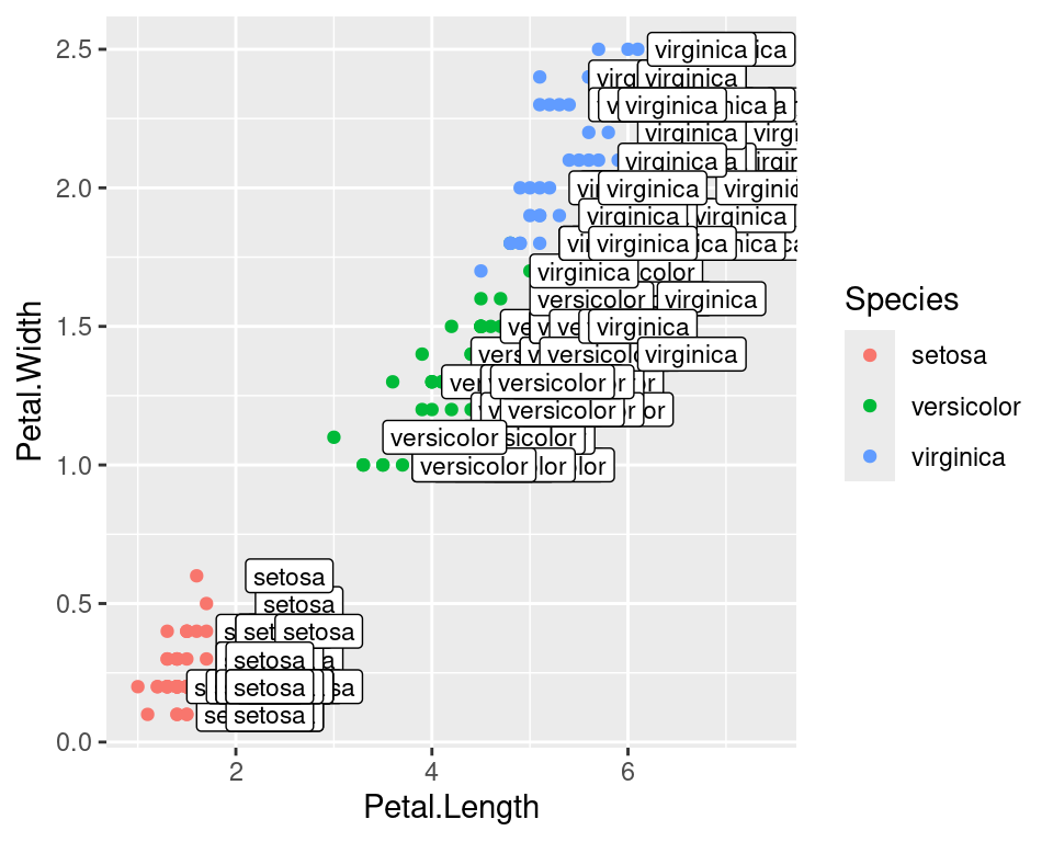
Check out the R package ggrepel allows for non-overlapping labels (here).
2.14 Annotations
Custom annotations of any geom can be added arbitrarily anywhere on the plot.
ggplot(data = iris, mapping = aes(x = Petal.Length, y = Petal.Width)) +
  geom_point(aes(color = Species)) +
  annotate("text", x = 2.5, y = 2.1, label = "There is a random line here") +
  annotate("segment", x = 2, xend = 4, y = 1.5, yend = 2)
2.15 Barplots
ggplot(data = iris, mapping = aes(x = Species, y = Petal.Width)) +
  geom_bar(stat = "identity")
2.16 Flip axes
x and y axes can be flipped using coord_flip.
ggplot(data = iris, mapping = aes(x = Species, y = Petal.Width)) +
  geom_bar(stat = "identity") +
  coord_flip()
2.17 Error Bars
An example of using error bars with points in few steps:
- The mean and standard deviation is computed.
- This is used to create upper and lower bounds for the error bars.
dfr <- iris %>%
  group_by(Species) %>%
  summarise(mean = mean(Sepal.Length), sd = sd(Sepal.Length)) %>%
  mutate(high = mean + sd, low = mean - sd)
dfr
ggplot(data = dfr, mapping = aes(x = Species, y = mean, color = Species)) +
  geom_point(size = 4) +
  geom_errorbar(aes(ymax = high, ymin = low), width = 0.2)
## # A tibble: 3 × 5
## Species mean sd high low
## <fct> <dbl> <dbl> <dbl> <dbl>
## 1 setosa 5.01 0.352 5.36 4.65
## 2 versicolor 5.94 0.516 6.45 5.42
## 3 virginica 6.59 0.636 7.22 5.95
3 Gene counts data
With a dataset like the gene-expression data, one would always want to look at the distribution of the counts between the samples. This can be done using a boxplot. Let’s create a boxplot of the counts.
3.1 Boxplot
ggplot(gene_counts_long) +
geom_boxplot(aes(x = Sample_Name, y = log10(counts + 1))) 
You can notice that the ggplot sorts the variables alpha-numerically, like in the case above with Sample_Name. One can convert that variable into a factor and specify the levels to control the order of that variable.
gene_counts_long$Sample_Name <- factor(gene_counts_long$Sample_Name,
  levels = c("t0_A","t0_B","t0_C","t2_A","t2_B","t2_C","t6_A","t6_B","t6_C","t24_A","t24_B","t24_C"))

ggplot(gene_counts_long) +
geom_boxplot(aes(x = Sample_Name, y = log10(counts + 1))) 
We can also additionally use the fill aesthetic to color the boxes based on the Time variable.
ggplot(gene_counts_long) +
geom_boxplot(aes(x = Sample_Name, y = log10(counts + 1), fill = Time)) 
3.2 Violin plot
ggplot(gene_counts_long) +
geom_violin(aes(x = Sample_Name, y = log10(counts + 1), fill = Time)) 
3.3 Errorbars
Below is an example of using creating se() function that calculates standard error and then using it to create a barplot with error bars.
se <- function(x) sqrt(var(x)/length(x))
gene_counts_long %>%
  group_by(Time) %>%
  summarise(mean=mean(log10(counts +1)),se=se(log10(counts +1))) %>%
  ggplot(aes(x=Time, y=mean, fill = Time)) +
  geom_col() +
  geom_errorbar(aes(ymax=mean+se,ymin=mean-se),width=0.2)
Notice that you can also send the data to ggplot() using the %>% operator. However, keep track of the commands related to tidyverse uses %>% and ggplot2 uses +.
3.4 Stacked bars
This is probably one of the plots that is not recommnded to use as it is hard to read and interpret. But it is still good to know how to create it.
gene_counts_long %>%
  group_by(Time, Replicate) %>%
  summarise(mean=mean(log10(counts +1)),se=se(log10(counts +1))) %>%
  ggplot(aes(x=Time, y=mean, fill = Replicate)) +
  geom_col(position = "stack")
probably a better way to show this information is to use a dodged barplot.
gene_counts_long %>%
  group_by(Time, Replicate) %>%
  summarise(mean=mean(log10(counts +1)),se=se(log10(counts +1))) %>%
  ggplot(aes(x=Time, y=mean, fill = Replicate)) +
  geom_col(position = "dodge")
3.5 Exercise
You can try to create a PCoA or an MDS plot from this dataset. Below is an example of how to create an MDS object.
gc_dist <- dist(t(gene_counts))
gc_mds <- cmdscale(gc_dist,eig=TRUE, k=2)
Some tips:
- Look at the
gc_mdsobject to see what it contains. You will need to convert it to a data frame. - Then add the sample information (metadata) to it using
left_join(). - Then you can use
ggplot()to create a scatter plot (aes(x = MDS1, y = MDS2)) of the two dimensions. - The mds object gc_mds has “eigenvalues”. You can calculate the variance of each co-ordinates (MDS1, MDS2) by
Variance <- Eigenvalues / sum(Eigenvalues)
4 Covid data
Covid cases data was download from ECDC as a CSV file. We will explore this dataset to plot some common scientific figures.
Read the table, keep only date up to september, convert the dateRep as date format to a new column named date, convert month and year to factors.
d <- read.csv("https://raw.githubusercontent.com/NBISweden/workshop-r/master/data/lab_ggplot2/covid.csv", header = TRUE, stringsAsFactors = TRUE) %>%
  filter(month <= 9) %>%
  mutate(
    date = as.Date(as.character(dateRep), "%d/%m/%Y"),
    month = as.factor(month),
    year = as.factor(year)
  )
as_tibble(d)
## # A tibble: 45,951 × 13
## dateRep day month year cases deaths countriesAndTerritories geoId
## <fct> <int> <fct> <fct> <int> <int> <fct> <fct>
## 1 30/09/2020 30 9 2020 15 2 Afghanistan AF
## 2 29/09/2020 29 9 2020 12 3 Afghanistan AF
## 3 28/09/2020 28 9 2020 0 0 Afghanistan AF
## 4 27/09/2020 27 9 2020 35 0 Afghanistan AF
## 5 26/09/2020 26 9 2020 6 2 Afghanistan AF
## 6 25/09/2020 25 9 2020 16 0 Afghanistan AF
## 7 24/09/2020 24 9 2020 25 5 Afghanistan AF
## 8 23/09/2020 23 9 2020 71 2 Afghanistan AF
## 9 22/09/2020 22 9 2020 30 3 Afghanistan AF
## 10 21/09/2020 21 9 2020 0 0 Afghanistan AF
## # ℹ 45,941 more rows
## # ℹ 5 more variables: countryterritoryCode <fct>, popData2019 <int>,
## # continentExp <fct>,
## # Cumulative_number_for_14_days_of_COVID.19_cases_per_100000 <dbl>,
## # date <date>4.1 Histogram
Create a histogram showing the overall distribution of cases.
d %>%
  ggplot(aes(x = cases)) +
  geom_histogram()
A whole lot of zero cases which is not surprising. A very few number of extremely large number of cases.
4.2 Line plot
A line plot is a good option when you dense data and over a time period/duration. Create a line plot for the Country Sweden (geoId=="SE" or countriesAndTerritories=="Sweden") showing date (date) on the x-axis and cases per day (cases) on the y-axis. Set a plot title and axes titles.
d %>%
  filter(geoId == "SE") %>%
  ggplot(aes(x = date, y = cases)) +
  geom_line() +
  labs(x = "Date", y = "Cases", title = "Sweden | COVID Cases Per Day")
The number of cases per day in Sweden are shown for the period from Jan to Sep. The highest peak is in June and cases were low in summer. Why do you think the line is oscillating up and down rather than being a smooth line?
Similar to above, create a line plot for the following 8 countries: Sweden, Denmark, Norway, Finland, United_Kingdom, France, Germany, Italy where each country has a different colored line. Set plot title and axes titles. Change theme to theme_bw().
d %>%
  filter(countriesAndTerritories %in% c("Sweden", "Denmark", "Norway", "Finland", "United_Kingdom", "France", "Germany", "Italy")) %>%
  ggplot(aes(x = date, y = cases, colour = countriesAndTerritories)) +
  geom_line() +
  scale_color_discrete(name = "Country") +
  labs(x = "Date", y = "Cases", title = "COVID Cases Per Day") +
  theme_bw()
The countries with lower number of counts are hard to see. Perhaps a log transformation would help? Change the y-axis to a log scale to bring clarity to countries with lower cases.
d %>%
  filter(countriesAndTerritories %in% c("Sweden", "Denmark", "Norway", "Finland", "United_Kingdom", "France", "Germany", "Italy")) %>%
  ggplot(aes(x = date, y = cases, colour = countriesAndTerritories)) +
  geom_line() +
  scale_y_log10() +
  scale_color_discrete(name = "Country") +
  labs(x = "Date", y = "Cases", title = "COVID Cases Per Day") +
  theme_bw()
Did that really help? Why not? Perhaps we could draw a trendline rather than showing the actual data. Create a line plot for the same information as above showing a smoothed trendline (geom_smooth()) rather than the actual data points.
d %>%
  filter(countriesAndTerritories %in% c("Sweden", "Denmark", "Norway", "Finland", "United_Kingdom", "France", "Germany", "Italy")) %>%
  ggplot(aes(x = date, y = cases, colour = countriesAndTerritories)) +
  geom_smooth() +
  scale_y_log10() +
  scale_color_discrete(name = "Country") +
  labs(x = "Date", y = "Cases", title = "COVID Cases Per Day") +
  theme_bw()
This is much easier to read.
Similarly, we can plot regression lines by changing arguments inside geom_smooth().
d %>%
  filter(countriesAndTerritories %in% c("Sweden", "Denmark", "Norway", "Finland", "United_Kingdom", "France", "Germany", "Italy")) %>%
  ggplot(aes(x = date, y = cases, colour = countriesAndTerritories)) +
  geom_smooth(method = "lm") +
  scale_y_log10() +
  scale_color_discrete(name = "Country") +
  labs(x = "Date", y = "Cases", title = "COVID Cases Per Day") +
  theme_bw()
4.3 Boxplots
Boxplot show the full distribution of data within a bin. Now, for the same countries, create monthwise boxplots (geom_boxplot()) of cases.
d %>%
  filter(countriesAndTerritories %in% c("Sweden", "Denmark", "Norway", "Finland", "United_Kingdom", "France", "Germany", "Italy")) %>%
  ggplot(aes(x = month, y = cases, colour = countriesAndTerritories)) +
  geom_boxplot() +
  scale_color_discrete(name = "Country") +
  labs(x = "Month", y = "Cases", title = "COVID Cases Per Month") +
  theme_bw()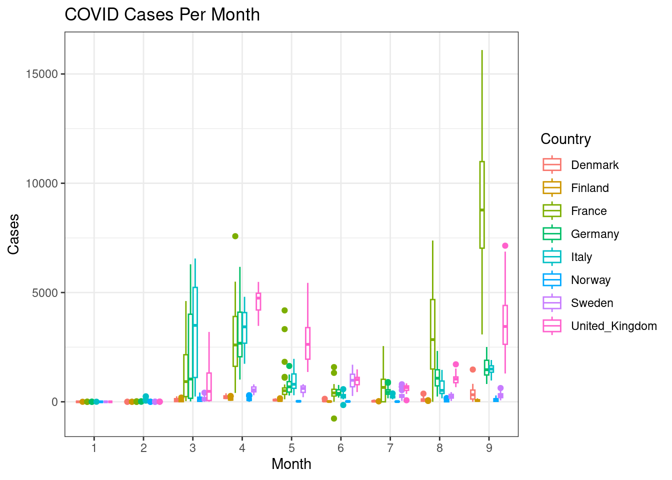
This gets a bit messy. Can you split each country into a subplot rather than showing all the countries in one plot?
d %>%
  filter(countriesAndTerritories %in% c("Sweden", "Denmark", "Norway", "Finland", "United_Kingdom", "France", "Germany", "Italy")) %>%
  ggplot(aes(x = month, y = cases, colour = countriesAndTerritories)) +
  geom_boxplot() +
  facet_wrap(~countriesAndTerritories) +
  scale_color_discrete(name = "Country") +
  labs(x = "Month", y = "Cases", title = "COVID Cases Per Month") +
  theme_bw()
4.4 Barplots
Create a barplot (geom_bar()) with mean cases for each continent.
d %>%
  group_by(continentExp) %>%
  summarise(mean = mean(cases, na.rm = TRUE)) %>%
  ggplot(aes(x = continentExp, y = mean)) +
  geom_bar(stat = "identity")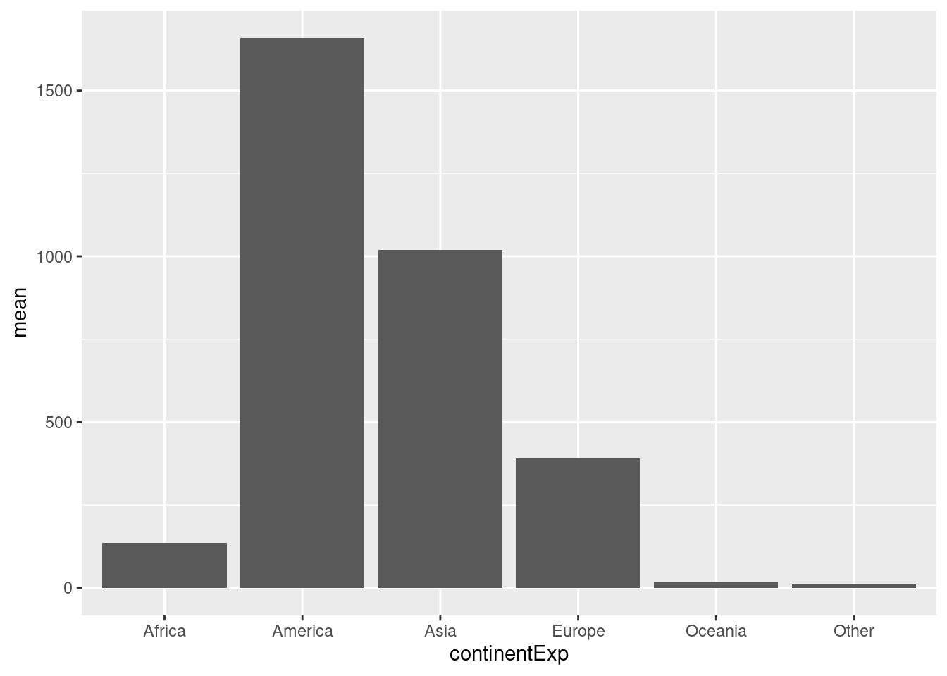
Now for a bit more complexity, create a stacked barplot (geom_bar()) with total cases monthwise for each continent. Set months on the x-axis, cases on the y-axis. Colour the bars by continent.
d %>%
  group_by(continentExp, month) %>%
  summarise(sum = sum(cases, na.rm = TRUE)) %>%
  ggplot(aes(x = month, y = sum, fill = continentExp)) +
  geom_bar(stat = "identity")
as_tibble(d)
## # A tibble: 45,951 × 13
## dateRep day month year cases deaths countriesAndTerritories geoId
## <fct> <int> <fct> <fct> <int> <int> <fct> <fct>
## 1 30/09/2020 30 9 2020 15 2 Afghanistan AF
## 2 29/09/2020 29 9 2020 12 3 Afghanistan AF
## 3 28/09/2020 28 9 2020 0 0 Afghanistan AF
## 4 27/09/2020 27 9 2020 35 0 Afghanistan AF
## 5 26/09/2020 26 9 2020 6 2 Afghanistan AF
## 6 25/09/2020 25 9 2020 16 0 Afghanistan AF
## 7 24/09/2020 24 9 2020 25 5 Afghanistan AF
## 8 23/09/2020 23 9 2020 71 2 Afghanistan AF
## 9 22/09/2020 22 9 2020 30 3 Afghanistan AF
## 10 21/09/2020 21 9 2020 0 0 Afghanistan AF
## # ℹ 45,941 more rows
## # ℹ 5 more variables: countryterritoryCode <fct>, popData2019 <int>,
## # continentExp <fct>,
## # Cumulative_number_for_14_days_of_COVID.19_cases_per_100000 <dbl>,
## # date <date>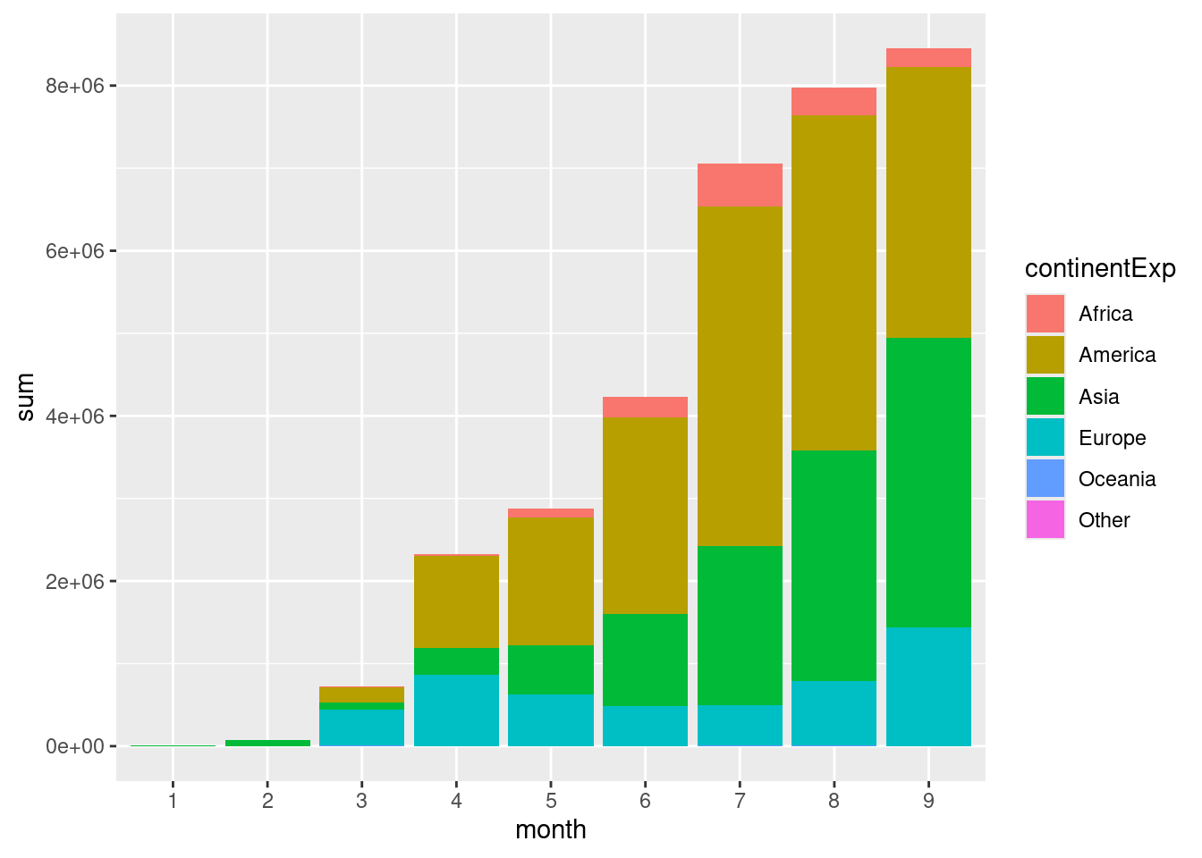
This figure shows the total number of cases per month across the globe. Continent-wise information shows that a large proportion of the cases are in America followed by Asia. The more common usage of stacked barplots is to show proportion/percentage rather than absolute counts (ie; all the bars are same height).
Create a stacked barplot as above showing proportion of total cases on the y-axis.
d %>%
  group_by(continentExp, month) %>%
  summarise(sum = sum(cases, na.rm = TRUE)) %>%
  group_by(month) %>%
  mutate(total = sum(sum, na.rm = TRUE), frac = round(sum / total, 5)) %>%
  ggplot(aes(x = month, y = frac, fill = continentExp)) +
  geom_bar(stat = "identity") +
  scale_fill_discrete(name = "Continent") +
  theme_bw() +
  labs(x = "Month", y = "Proportion of Cases")
Now, we can see that the pandemic initially started with 100% of the cases in the Asia. As we can also see the rise and fall of cases over summer.
Now let’s look at barplots with error bars. - First, create a barplot showing mean number of cases per continent per month. - Second, place the bars within a group (month) next to each other rather than stack.
d %>%
  group_by(continentExp, month) %>%
  summarise(mean = mean(cases, na.rm = TRUE)) %>%
  ggplot(aes(x = month, y = mean, fill = continentExp)) +
  geom_bar(stat = "identity", position = position_dodge()) +
  scale_fill_discrete(name = "Continent") +
  labs(x = "Month", y = "Mean cases per Month")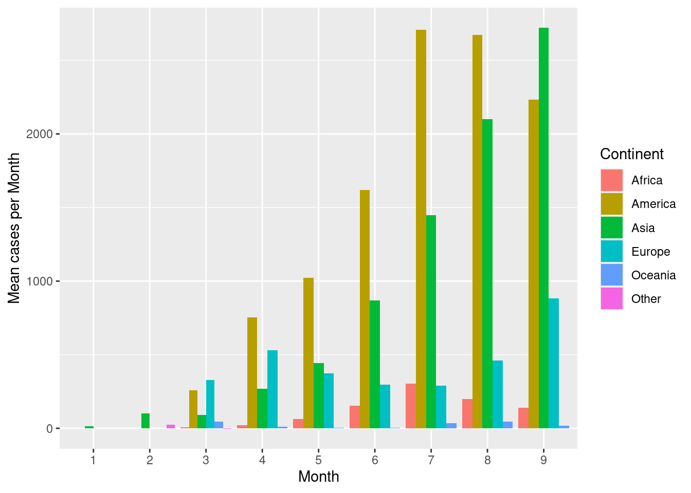
Now to compute, error bars, computer error metrics in the summary() function, let’s say standard deviation (sd()).
d %>%
  group_by(continentExp, month) %>%
  summarise(
    mean = mean(cases, na.rm = TRUE),
    sd = sd(cases, na.rm = TRUE),
    high = mean + sd,
    low = mean - sd
  ) %>%
  ggplot(aes(x = month, y = mean, fill = continentExp)) +
  geom_bar(stat = "identity", position = position_dodge()) +
  geom_errorbar(aes(ymax = high, ymin = low), position = position_dodge(), colour = "grey40") +
  scale_fill_discrete(name = "Continent") +
  labs(x = "Month", y = "Mean cases per Month")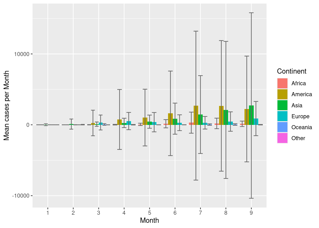
4.5 Scatterplots
Scatterplots are commonly used for continuous vs continuous variables. Let’s try to see if there is any relationship between number of cases and number of deaths. Create a scatterplot showing cases vs deaths.
ggplot(d, aes(cases, deaths)) +
  geom_point()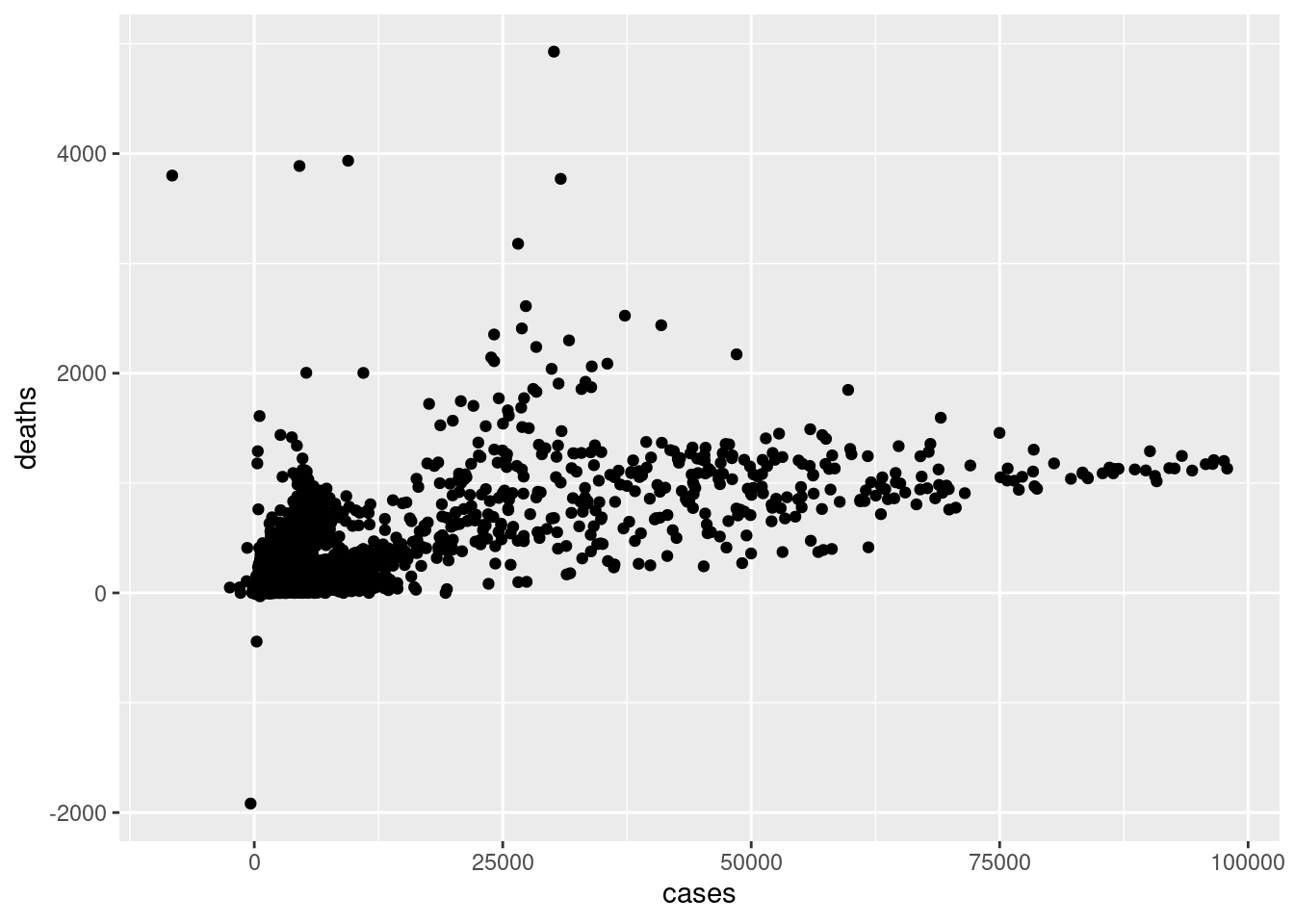
Scatterplots are extremely useful in visually inspecting relationships between variables.
Scatterplots can also be used with categorical variables. Create a scatterplot with month on the x-axis and cases per month on the y-axis. Color the points by continent.
ggplot(d, aes(x = month, y = cases, colour = continentExp)) +
  geom_point() +
  scale_colour_discrete(name = "Continent") +
  labs(x = "Month", y = "Cases per Month")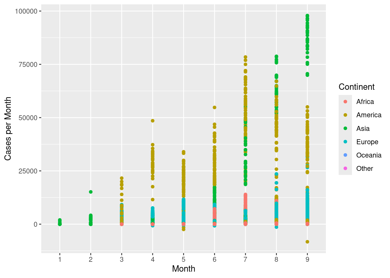
geom_jitter() can be used to jitter the points around, so they do not overlap.
ggplot(d, aes(x = month, y = cases, colour = continentExp)) +
  geom_jitter(width = 0.3) +
  scale_colour_discrete(name = "Continent") +
  labs(x = "Month", y = "Cases per Month")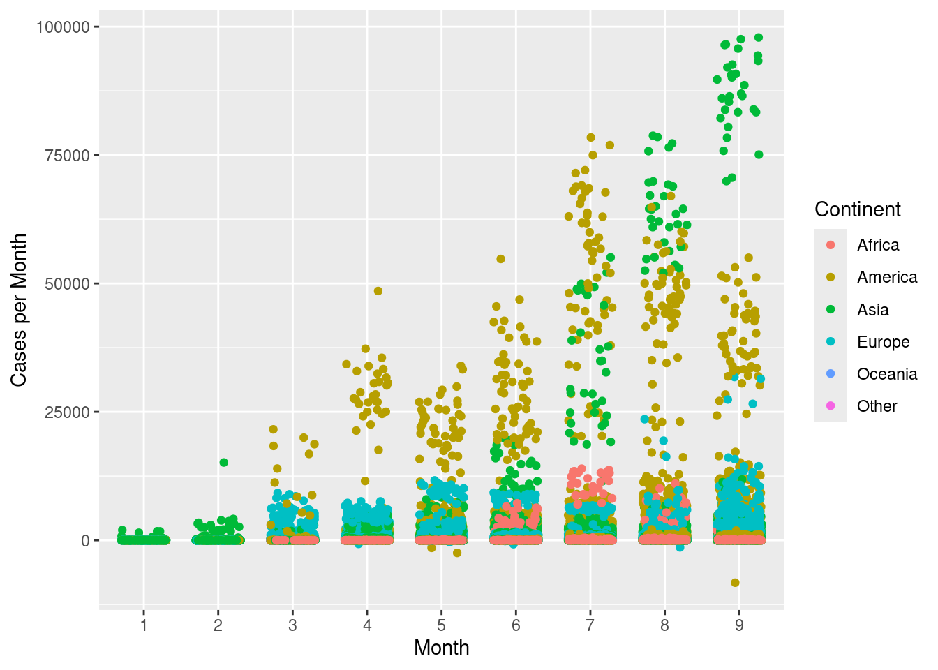
Create a scatterplot with month on the x-axis and mean cases per month on the y-axis. Color the points by continent.
d %>%
  group_by(month, continentExp) %>%
  summarise(mean = mean(cases, na.rm = TRUE)) %>%
  ggplot(aes(x = month, y = mean, colour = continentExp)) +
  geom_point() +
  scale_colour_discrete(name = "Continent") +
  labs(x = "Month", y = "Mean cases per Month")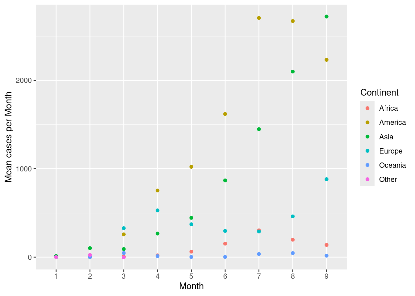
Add a line to connect the continents across months. Use the group argument in aes().
d %>%
  group_by(month, continentExp) %>%
  summarise(mean = mean(cases, na.rm = TRUE)) %>%
  ggplot(aes(x = month, y = mean, colour = continentExp, group = continentExp)) +
  geom_point() +
  geom_line() +
  scale_colour_discrete(name = "Continent") +
  labs(x = "Month", y = "Mean cases per Month")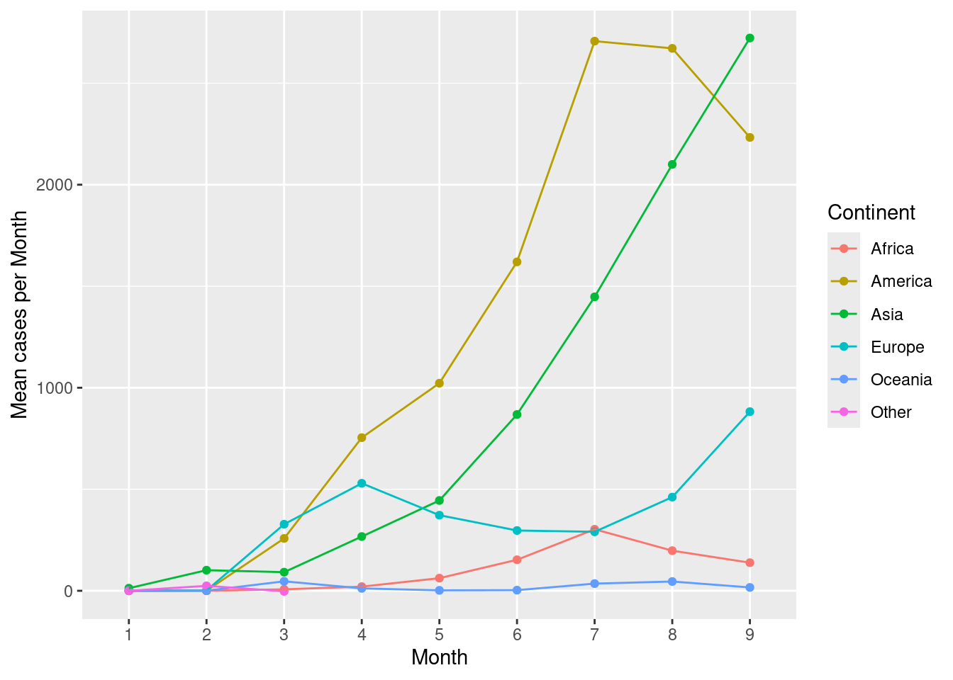
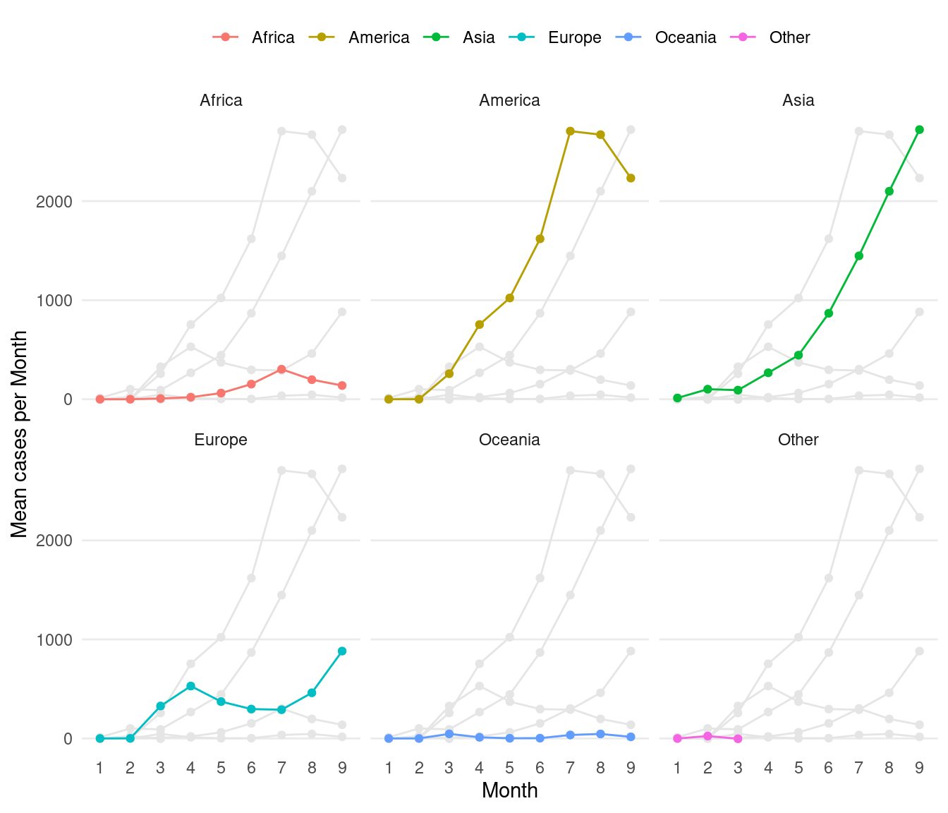
Now for a slightly more advanced example. Create the same plot above with each continent as separate facets. Add all other continents in the background as reference lines in light grey colour.
ds <- d %>%
  group_by(month, continentExp) %>%
  summarise(mean = mean(cases, na.rm = TRUE))

# new df for background points
dsb <- ds %>%
  mutate(co = continentExp) %>%
  select(-continentExp)

ggplot() +
  geom_point(data = dsb, aes(x = month, y = mean, group = co), colour = "grey90") +
  geom_line(data = dsb, aes(x = month, y = mean, group = co), colour = "grey90") +
  geom_point(data = ds, aes(x = month, y = mean, colour = continentExp, group = continentExp)) +
  geom_line(data = ds, aes(x = month, y = mean, colour = continentExp, group = continentExp)) +
  facet_wrap(~continentExp) +
  scale_colour_discrete(name = "Continent") +
  labs(x = "Month", y = "Mean cases per Month") +
  guides(colour = guide_legend(nrow = 1)) +
  theme_bw() +
  theme(
    plot.background = element_blank(),
    panel.border = element_blank(),
    axis.ticks = element_blank(),
    panel.grid.minor = element_blank(),
    panel.grid.major.x = element_blank(),
    legend.position = "top",
    legend.direction = "horizontal",
    legend.title = element_blank(),
    strip.background = element_blank()
  )
4.6 Heatmap
Here, we will look at creating a heatmap using ggplot2 as well as fine customisation of the plot for publication. This heatmap shows cases for all European countries over time. This is also a slightly more advanced example.
First, countries in Europe are selected and cases per million people is computed.
# subset europe, calculate cases per million
d2 <- d %>%
  filter(continentExp == "Europe") %>%
  mutate(casesp = log10(round((cases / popData2019) * 10^6, 3) + 1))
# colours
cols <- c("#e7f0fa", "#c9e2f6", "#95cbee", "#0099dc", "#4ab04a", "#ffd73e", "#eec73a", "#e29421", "#f05336", "#ce472e")
leg_label <- "Log[10]~Cases~Per~Million~Persons"
# plotting
ggplot(d2, aes(x = date, y = countriesAndTerritories, fill = casesp)) +
geom_tile() +
labs(x = "", y = "") +
scale_fill_gradientn(
colors = cols, na.value = "grey90",
guide = guide_colourbar(ticks = T, nbin = 10, barheight = .5, label = T, barwidth = 10),
name = eval(parse(text = leg_label))
) +
scale_x_date(
breaks = seq(as.Date("2020/1/1"), by = "month", length.out = 10),
labels = format(seq(as.Date("2020/1/1"), by = "month", length.out = 10), "%b")
) +
theme_bw() +
theme(
plot.background = element_blank(),
panel.border = element_blank(),
axis.ticks = element_blank(),
panel.grid.minor = element_blank(),
panel.grid.major = element_blank(),
legend.position = "top",
legend.direction = "horizontal"
)
# pheatmap::pheatmap(d3,cluster_cols = F,scale = "none")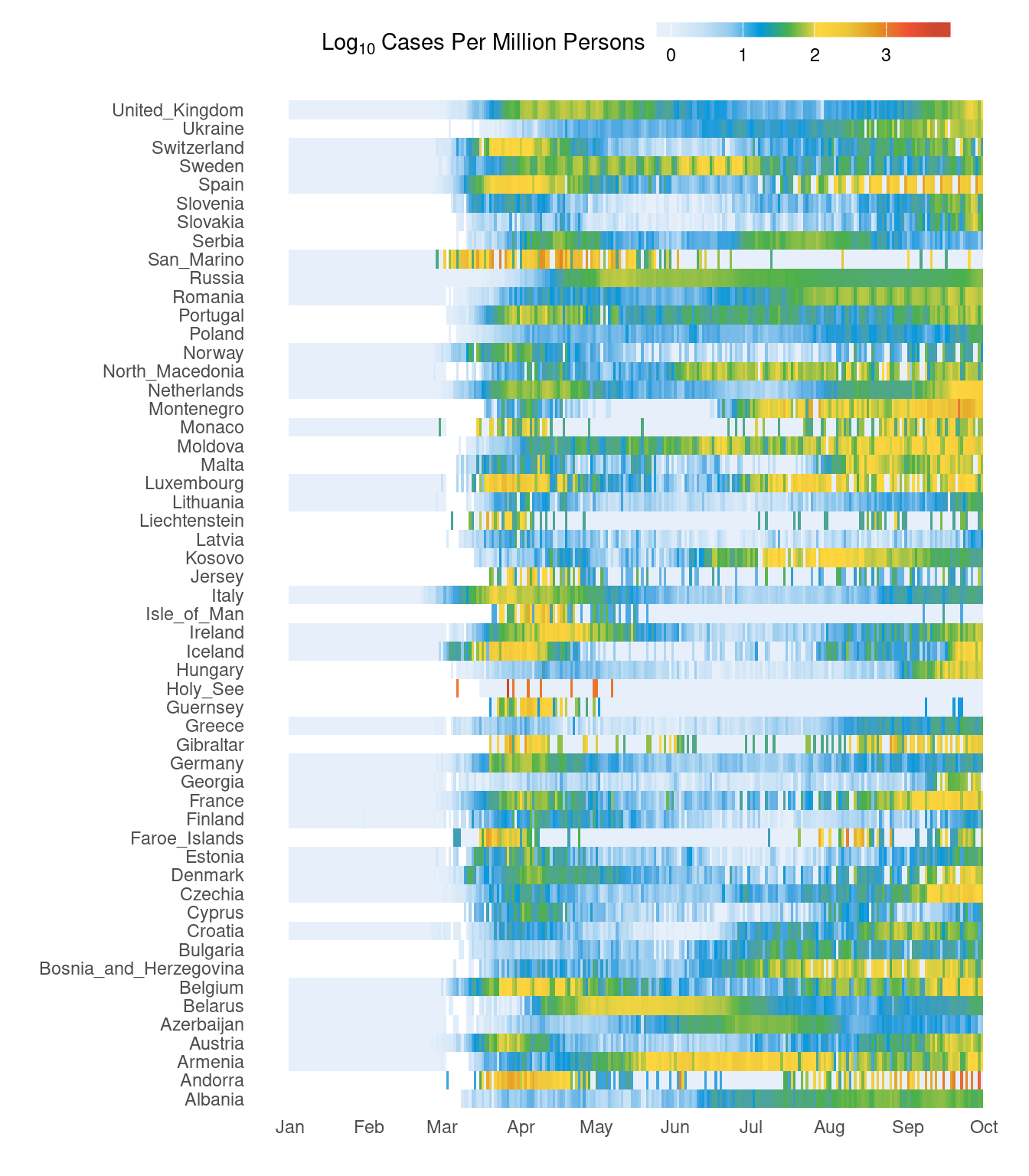
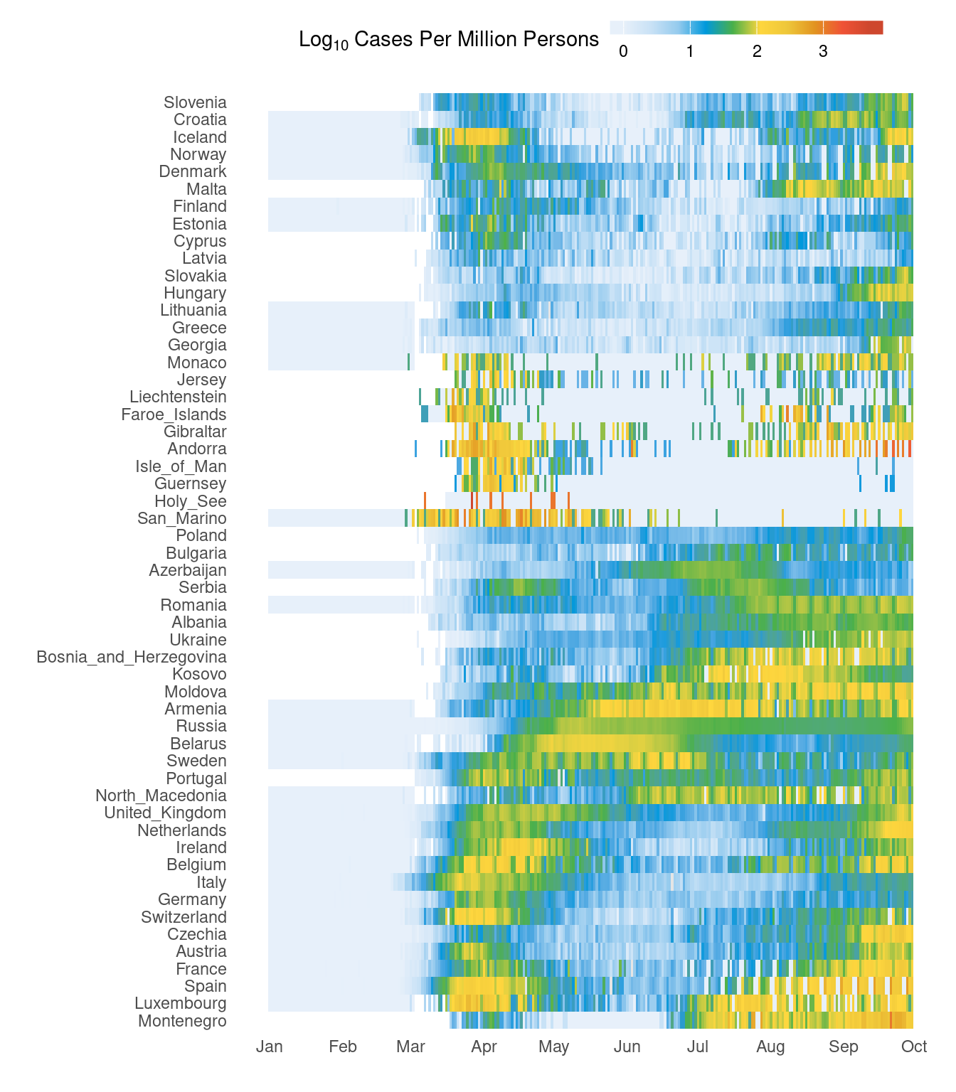
It would be nice to have the countries grouping together based on the trend rather than just alphabetical order. This bit of code below clusters countries based on the data. Therefore, countries with similar case patterns should cluster together.
# cluster countries
d3 <- d2 %>%
  mutate(casesp = casesp) %>%
  select(date, countriesAndTerritories, casesp) %>%
  spread(key = date, value = casesp)
rownames(d3) <- d3$countriesAndTerritories
d3$countriesAndTerritories <- NULL
h <- hclust(dist(d3))
d2$countriesAndTerritories <- factor(as.character(d2$countriesAndTerritories), levels = rownames(d3)[h$order])
Now, our new figure looks like this. It should be easier to see the trend over time. Primary and secondary waves are now starting to be easily visible.
# colours
cols <- c("#e7f0fa", "#c9e2f6", "#95cbee", "#0099dc", "#4ab04a", "#ffd73e", "#eec73a", "#e29421", "#f05336", "#ce472e")
leg_label <- "Log[10]~Cases~Per~Million~Persons"

# plotting
ggplot(d2, aes(x = date, y = countriesAndTerritories, fill = casesp)) +
  geom_tile() +
  labs(x = "", y = "") +
  scale_fill_gradientn(
    colors = cols, na.value = "grey90",
    guide = guide_colourbar(ticks = T, nbin = 10, barheight = .5, label = T, barwidth = 10),
    name = eval(parse(text = leg_label))
  ) +
  scale_x_date(
    breaks = seq(as.Date("2020/1/1"), by = "month", length.out = 10),
    labels = format(seq(as.Date("2020/1/1"), by = "month", length.out = 10), "%b")
  ) +
  theme_bw() +
  theme(
    plot.background = element_blank(),
    panel.border = element_blank(),
    axis.ticks = element_blank(),
    panel.grid.minor = element_blank(),
    panel.grid.major = element_blank(),
    legend.position = "top",
    legend.direction = "horizontal"
  )
5 Cheatsheet
5.1 General
| Function / Layer | Purpose | Example |
|---|---|---|
ggplot() |
Initialize a plot; specify data + aesthetics. | ggplot(df, aes(x, y)) |
aes() |
Map variables to visual properties (x, y, color…). | aes(x = age, y = height, color = group) |
geom_point() |
Scatterplot points. | geom_point(size = 3) |
geom_line() |
Line plot. | geom_line() |
geom_col() |
Bar plot with heights from data. | geom_col() |
geom_bar() |
Bar count plot. | geom_bar() |
geom_histogram() |
Histogram of one numeric variable. | geom_histogram(bins = 30) |
geom_boxplot() |
Boxplot. | geom_boxplot() |
geom_violin() |
Violin plot. | geom_violin() |
geom_smooth() |
Add trend line (linear, loess…). | geom_smooth(method = "lm") |
geom_text() |
Add text labels. | geom_text(aes(label = name)) |
geom_label() |
Text labels with a box. | geom_label(aes(label = value)) |
labs() |
Titles and axis labels. | labs(title="Title", x="Time", y="Value") |
ggtitle() |
Add a main title. | ggtitle("My Plot") |
xlab(), ylab() |
Axis labels. | xlab("Time") |
scale_x_continuous() |
Custom x-axis scale. | scale_x_continuous(limits = c(0, 10)) |
scale_y_continuous() |
Custom y-axis scale. | scale_y_continuous(trans = "log10") |
scale_color_manual() |
Custom colors for categories. | scale_color_manual(values = c("red","blue")) |
facet_wrap() |
Split plot into multiple panels (1 variable). | facet_wrap(~ species) |
facet_grid() |
Grid of panels (2 variables). | facet_grid(sex ~ species) |
theme() |
Modify plot appearance. | theme_minimal() |
theme_minimal() |
Minimal white theme. | + theme_minimal() |
theme_bw() |
Black-and-white theme. | + theme_bw() |
theme_classic() |
Classic theme. | + theme_classic() |
coord_flip() |
Flip axes. | coord_flip() |
coord_cartesian() |
Zoom in without removing data. | coord_cartesian(xlim=c(0,10)) |
element_text() |
Modify text inside a theme. | theme(axis.text.x = element_text(angle=45)) |
guides() |
Control legends. | guides(color = "none") |
ggsave() |
Save a plot to file. | ggsave("plot.png", width=5, height=4) |
5.2 Coordinate Systems
| Function | What it does | Common use / Example |
|---|---|---|
coord_cartesian() |
Adjusts the visible region without removing data | coord_cartesian(xlim = c(2, 8)) → zoom into x-range 2–8 |
coord_fixed() |
Keeps equal aspect ratio for x and y | Useful for maps or shapes where scale should be equal |
coord_flip() |
Swaps x and y axes | Great for horizontal bar plots |
coord_trans() |
Transforms axes (e.g., log, sqrt) | coord_trans(y = "log10") |
coord_polar() |
Converts to polar coordinates | Create pie charts or circular plots |
coord_map() |
Uses map projection (scales adjusted for geography) | Plot geographic data with correct proportions |