command1 Introduction
RNA-seq has become a powerful approach to study the continually changing cellular transcriptome. Here, one of the most common questions is to identify genes that are differentially expressed between two conditions, e.g. controls and treatment. The main exercise in this tutorial will take you through a basic bioinformatic analysis pipeline to answer just that, it will show you how to find differentially expressed (DE) genes.
Main exercise
- Check the quality of the raw reads with FastQC
- Map the reads to the reference genome using HISAT2
- Assess the post-alignment quality using Qualimap
- Count the reads overlapping with genes using featureCounts
- Find DE genes using DESeq2 in R
- RNA-Seq figures and plots using R
RNA-seq experiment does not necessarily end with a list of DE genes. If you have time after completing the main exercise, try one (or more) of the bonus exercises. The bonus exercises can be run independently of each other, so choose the one that matches your interest. Bonus sections are listed below.
Bonus exercises
- Functional annotation of DE genes using GO database
- Visualisation of RNA-seq BAM files using IGV genome browser
General guide
In code and paths, remember to change username with your actual HPC username.
You are welcome to try your own solutions to the problems, before checking the solution. Click the button to see the suggested solution. There is more than one way to complete a task. Discuss with person next to you and ask us when in doubt.
Input code blocks are displayed like shown below.
2 Data description
The data used in this exercise is from the paper: Poitelon, Yannick, et al. YAP and TAZ control peripheral myelination and the expression of laminin receptors in Schwann cells. Nature neuroscience 19.7 (2016): 879. In this study, YAP and TAZ genes were knocked-down in Schwann cells to study myelination, using mice as a model.
Myelination is essential for nervous system function. Schwann cells are a type of glial cell that interact with neurons and the basal lamina to myelinate axons. Myelinated axons transfer signals up to 10x faster. Hippo pathway is a conserved pathway involved in cell contact inhibition, and it acts to promote cell proliferation and inhibits apoptosis. Transcription co-activators YAP and TAZ are two major downstream effectors of the Hippo pathway, and have redundant roles in transcriptional activation. TAZ and YAP genes were knocked-down to study their effect on neurons.
The material for RNA-seq was collected from 2 conditions (Wt and KO), each with 3 biological replicates.
| Accession | Condition | Replicate |
|---|---|---|
| SRR3222409 | KO | 1 |
| SRR3222410 | KO | 2 |
| SRR3222411 | KO | 3 |
| SRR3222412 | Wt | 1 |
| SRR3222413 | Wt | 2 |
| SRR3222414 | Wt | 3 |
Note
For the purpose of this tutorial, to shorten the time needed to run various bioinformatics steps, we have picked reads for a single chromosome (Chr 19) and downsampled the reads. We randomly sampled, without replacement, 25% reads from each sample, using fastq-sample from the toolset fastq-tools.
3 Main exercise
The main exercise covers Differential Gene Expression (DGE) workflow from raw reads to a list of differentially expressed genes.
3.1 Using HPC
Use ThinLinc
If you have issues opening GUI windows from HPC through the terminal, you can use ThinLinc.
If you are not on ThinLinc, connect to HPC first. For instructions, see Contents > Connecting to HPC. Remember to replace username.
ssh -XY username@dardel.pdc.kth.seBook a node.
For the RNA-Seq part of the course, we will work on the HPC. The code below is valid to run at the start of the day. If you are running it in the middle of a day, you need to decrease the time (-t). Do not run this twice and also make sure you are not running computations on a login node.
Book compute resources for RNA-Seq lab.
Tip
The --reservation is only used during the workshop and not needed when working on your projects. Use edu26-03-05 for Thursday and edu26-03-06 for Friday.
salloc -A naiss2026-4-45 --reservation=edu26-03-05 -t 03:00:00 -p shared -c 4 --no-shellCheck allocation. Remember to replace username.
squeue -u usernameOnce allocation is granted, log on to the compute node. Remember to replace nodename.
ssh -Y nodename3.1.1 Set-up directory
Setting up the directory structure is an important step as it helps to keep our raw data, intermediate data and results in an organised manner. We suggest a location for the whole workshop (/cfs/klemming/projects/supr/naiss2026-4-45/username).
Within that, create a directory named rnaseq.
cd /cfs/klemming/projects/supr/naiss2026-4-45/username
mkdir rnaseq
Create the directory structure as shown below.
/cfs/klemming/projects/supr/naiss2026-4-45/username/
rnaseq/
  +-- 1_raw/
  +-- 2_fastqc/
  +-- 3_mapping/
  +-- 4_qualimap/
  +-- 5_dge/
  +-- 6_multiqc/
  +-- reference/
  |   +-- mouse_chr19_hisat2/
  +-- scripts/
cd rnaseq
mkdir 1_raw 2_fastqc 3_mapping 4_qualimap 5_dge 6_multiqc reference scripts reference/mouse_chr19_hisat2The 1_raw directory will hold the raw fastq files. 2_fastqc will hold FastQC outputs. 3_mapping will hold the mapping output files. 4_qualimap will hold the post alignment QC output. 5_dge will hold the counts from featureCounts and all differential gene expression related files. 6_multiqc will hold MultiQC outputs. reference directory will hold the reference genome, annotations and aligner indices.
Tip
It might be a good idea to open an additional terminal window. One to navigate through directories and another for scripting in the scripts directory.
3.1.2 Create symbolic links
We have the raw fastq files in this remote directory: /sw/courses/ngsintro/rnaseq/dardel/main/1_raw/. We are going to create symbolic links (soft-links) for these files from our 1_raw directory to the remote directory. We do this because fastq files tend to be large files and simply copying them would use up a lot of storage space. Soft-linking files and folders allows us to work with those files as if they were actually there.
Change to 1_raw directory. Use pwd to check if you are standing in the correct directory.
cd 1_raw
pwd/cfs/klemming/projects/supr/naiss2026-4-45/username/rnaseq/1_rawRun below to create softlinks. Note that the command ends in a space followed by a period.
ln -s /sw/courses/ngsintro/rnaseq/dardel/main/1_raw/*.gz .Check if your files have linked correctly. You should be able to see as below.
ls -lSRR3222409-19_1.fq.gz -> /sw/courses/ngsintro/rnaseq/main/1_raw/SRR3222409-19_1.fq.gz
SRR3222409-19_2.fq.gz -> /sw/courses/ngsintro/rnaseq/main/1_raw/SRR3222409-19_2.fq.gz
SRR3222410-19_1.fq.gz -> /sw/courses/ngsintro/rnaseq/main/1_raw/SRR3222410-19_1.fq.gz
SRR3222410-19_2.fq.gz -> /sw/courses/ngsintro/rnaseq/main/1_raw/SRR3222410-19_2.fq.gz
SRR3222411-19_1.fq.gz -> /sw/courses/ngsintro/rnaseq/main/1_raw/SRR3222411-19_1.fq.gz
SRR3222411-19_2.fq.gz -> /sw/courses/ngsintro/rnaseq/main/1_raw/SRR3222411-19_2.fq.gz
SRR3222412-19_1.fq.gz -> /sw/courses/ngsintro/rnaseq/main/1_raw/SRR3222412-19_1.fq.gz
SRR3222412-19_2.fq.gz -> /sw/courses/ngsintro/rnaseq/main/1_raw/SRR3222412-19_2.fq.gz
SRR3222413-19_1.fq.gz -> /sw/courses/ngsintro/rnaseq/main/1_raw/SRR3222413-19_1.fq.gz
SRR3222413-19_2.fq.gz -> /sw/courses/ngsintro/rnaseq/main/1_raw/SRR3222413-19_2.fq.gz
SRR3222414-19_1.fq.gz -> /sw/courses/ngsintro/rnaseq/main/1_raw/SRR3222414-19_1.fq.gz
SRR3222414-19_2.fq.gz -> /sw/courses/ngsintro/rnaseq/main/1_raw/SRR3222414-19_2.fq.gz3.2 Read QC
Quality check using FastQC
After receiving raw reads from a high throughput sequencing centre it is essential to check their quality. FastQC provides a simple way to do some quality control check on raw sequence data. It provides a modular set of analyses which you can use to get a quick impression of whether your data has any problems of which you should be aware before doing any further analysis.
Change into the 2_fastqc directory. Use pwd to check if you are standing in the correct directory.
cd ../2_fastqc
pwd/cfs/klemming/projects/supr/naiss2026-4-45/username/rnaseq/2_fastqcLoad module FastQC.
module load PDC/24.11
module load fastqc/0.12.1
Once the module is loaded, FastQC program is available through the command fastqc. Use fastqc --help to see the various parameters available to the program. We will use -o to specify the output directory path and finally, the name of the input fastq file to analyse. The syntax to run one file will look like below.
Don’t run this. It’s just a template.
fastqc -o . ../1_raw/filename.fq.gzBased on the above command, we will write a bash loop script to process all fastq files in the directory. Writing multi-line commands through the terminal can be a pain. Therefore, we will run larger scripts from a bash script file. Create a new file named fastqc.sh in your scripts directory.
touch ../scripts/fastqc.sh
ls -l ../scripts/
Use a text editor (nano,Emacs, gedit etc.) to edit fastqc.sh.
gedit behaves like a regular text editor with a standard graphical interface.
gedit ../scripts/fastqc.sh &Then add the lines below and save the file.
#!/bin/bash

module load PDC/24.11
module load fastqc/0.12.1

for i in ../1_raw/*.gz
do
    echo "Running $i ..."
    fastqc -o . "$i"
done
This script loops through all files ending in .gz. In each iteration of the loop, it executes fastqc on the file. The -o . flag to fastqc indicates that the output must be exported in this current directory (ie; the directory where this script is run).
In the 2_fastqc directory, run the script file fastqc.sh. Use pwd to check if you are standing in the correct directory.
bash ../scripts/fastqc.shAfter the fastqc run, there should be a .zip file and a .html file for every fastq file. The .html file is the report that you need. Download the .html files to your computer and open them in a web browser. You do not need to necessarily look at all files now. We will do a comparison with all samples when using the MultiQC tool.
Run this step in a LOCAL terminal and NOT on HPC. Open a terminal locally on your computer, move to a suitable download directory and run the command below to download one html report.
Remember to replace username.
scp username@dardel.pdc.kth.se:/cfs/klemming/projects/supr/naiss2026-4-45/username/rnaseq/2_fastqc/SRR3222409-19_1_fastqc.html .or download the whole directory.
scp -r username@dardel.pdc.kth.se:/cfs/klemming/projects/supr/naiss2026-4-45/username/rnaseq/2_fastqc .
Downloading using a GUI
Go back to the FastQC website and compare your report with the sample report for Good Illumina data and Bad Illumina data.
Discuss based on your reports, whether your data is of good enough quality and/or what steps are needed to fix it.
3.2.1 Questions
Why would the per-base sequence quality decrease towards the 3’ end of reads?
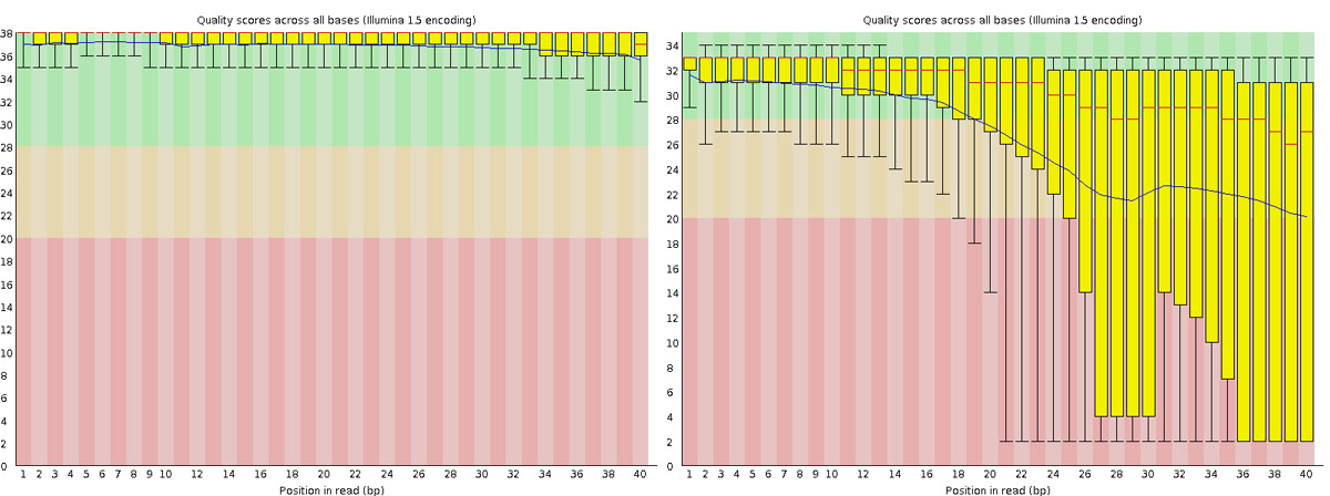
Answer
This is due to the chemistry of sequencing-by-synthesis. As the sequencing reaction progresses, nucleotide incorporation becomes less efficient, polymerase fidelity decreases, and phasing/pre-phasing errors accumulate. Signal decay and cross-talk between clusters also increase over longer run times. This used to be a normal characteristic of Illumina sequencing and is one of the reasons why the 3’ ends of reads are often quality trimmed before downstream analysis.
What does a bimodal distribution in the “Per sequence GC content” plot indicate, and what could cause it?
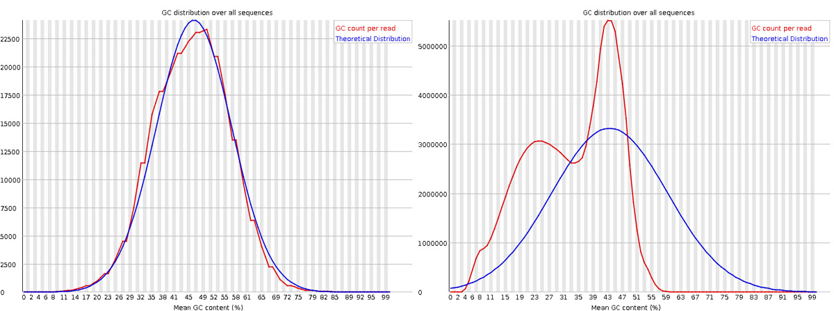
Answer
A bimodal GC distribution suggests contamination with sequences from a different organism or source with a distinct GC content. Common causes include: (1) rRNA contamination (rRNA has different GC content than mRNA), (2) adapter dimers, (3) sample contamination from another species, or (4) contamination with spike-in controls. In RNA-seq, this might also indicate incomplete rRNA depletion or poly-A selection issues.
Why might you see overrepresented sequences in your FastQC report, and when should you be concerned?
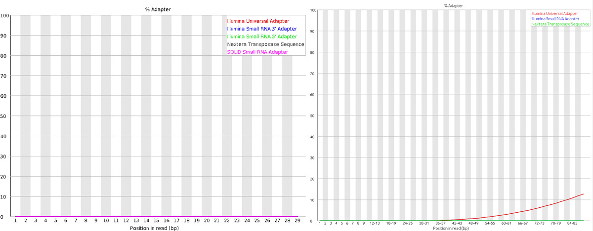
Answer
Overrepresented sequences can arise from: (1) rRNA contamination (common in RNA-seq), (2) adapter sequences that weren’t properly trimmed, (3) highly expressed genes (expected in RNA-seq), (4) PCR duplicates from low complexity libraries, or (5) technical artifacts. You should be concerned if overrepresented sequences are adapters (indicates trimming issues) or if they constitute a very large fraction of reads. However, seeing some highly expressed housekeeping genes or tissue-specific genes as overrepresented is normal in RNA-seq experiments.
In RNA-seq, why is it normal to see high sequence duplication levels?
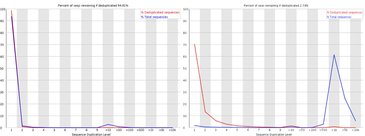
Answer
Unlike DNA sequencing where each fragment should be unique, RNA-seq inherently has duplication due to biological variation in gene expression levels. Highly expressed genes will naturally generate many identical reads. FastQC was originally designed for genomic DNA sequencing where high duplication indicates PCR bias. In RNA-seq, high duplication levels are expected and reflect the transcriptome’s dynamic range. However, extremely high duplication (>90%) combined with low library complexity might still indicate problematic library preparation.
How would you determine if your RNA-seq library preparation included an rRNA depletion step or poly-A selection based on FastQC results?
Answer
You can look for: (1) Overrepresented sequences - check if ribosomal RNA sequences appear (indicates incomplete rRNA depletion), (2) GC content distribution - rRNA has a specific GC profile that would cause deviations, (3) After mapping, check the percentage of reads mapping to rRNA genes. Poly-A selection libraries typically show lower rRNA contamination but may miss non-polyadenylated transcripts. rRNA depletion maintains non-polyadenylated RNAs but may have higher rRNA background.
3.3 Mapping
Mapping reads using HISAT2
After verifying that the quality of the raw sequencing reads is acceptable, we will map the reads to the reference genome. There are many mappers/aligners available, so it may be good to choose one that is adequate for your type of data. Here, we will use a software called HISAT2 (Hierarchical Indexing for Spliced Alignment of Transcripts) as it is a good general purpose splice-aware aligner. It is fast and does not require a lot of RAM. Before we begin mapping, we need to obtain genome reference sequence (.fasta file) and build an aligner index. Due to time constraints, we will build an index only on chromosome 19.
3.3.1 Get reference
It is best if the reference genome (.fasta) and annotation (.gtf) files come from the same source to avoid potential naming conventions problems. It is also good to check in the manual of the aligner you use for hints on what type of files are needed to do the mapping. We will not be using the annotation (.gtf) during mapping, but we will use it during quantification.
What is the idea behind building an aligner index? What files are needed to build one? Where do we take them from? Could one use an index that was generated for another project? Check out the HISAT2 manual indexer section for answers. Browse through Ensembl and try to find the files needed. Note that we are working with Mouse (Mus musculus).
Move into the reference directory and download the Chr 19 genome (.fasta) file and the genome-wide annotation file (.gtf) from Ensembl.
You should be standing here to run this:
/cfs/klemming/projects/supr/naiss2026-4-45/username/rnaseq/referenceYou are most likely to use the latest version of ensembl release genome and annotations when starting a new analysis. For this exercise, we will choose ensembl version 99.
wget ftp://ftp.ensembl.org/pub/release-99/fasta/mus_musculus/dna/Mus_musculus.GRCm38.dna.chromosome.19.fa.gz
wget ftp://ftp.ensembl.org/pub/release-99/gtf/mus_musculus/Mus_musculus.GRCm38.99.gtf.gz
Decompress the files for use.
gunzip Mus_musculus.GRCm38.dna.chromosome.19.fa.gz
gunzip Mus_musculus.GRCm38.99.gtf.gz
From the full gtf file, we will also extract chr 19 alone to create a new gtf file for use later.
cat Mus_musculus.GRCm38.99.gtf | grep -E "^#|^19" > Mus_musculus.GRCm38.99-19.gtf The grep command is set to use regular expression with the -E argument. And it’s looking for lines starting with # or 19. # fetches the header and comments while 19 denotes all rows with annotations for chromosome 19.
Check what you have in your directory.
ls -ldrwxrwsr-x 2 user gXXXXXXX 4.0K Jan 22 21:59 mouse_chr19_hisat2
-rw-rw-r-- 1 user gXXXXXXX 26M Jan 22 22:46 Mus_musculus.GRCm38.99-19.gtf
-rw-rw-r-- 1 user gXXXXXXX 771M Jan 22 22:10 Mus_musculus.GRCm38.99.gtf
-rw-rw-r-- 1 user gXXXXXXX 60M Jan 22 22:10 Mus_musculus.GRCm38.dna.chromosome.19.fa3.3.2 Build index
Load module hisat2.
module load PDC/24.11
module load hisat2/2.2.1
To search for the tool or other versions of a tool, use module spider hisat.
Create a new bash script in your scripts directory named hisat2_index.sh and add the following lines:
#!/bin/bash

# load module
module load PDC/24.11
module load hisat2/2.2.1

hisat2-build \
  -p 1 \
  Mus_musculus.GRCm38.dna.chromosome.19.fa \
  mouse_chr19_hisat2/mouse_chr19_hisat2
The above script builds a HISAT2 index using the command hisat2-build. It should use 1 core for computation. The paths to the FASTA (.fa) genome file is specified. And the output path is specified. The output describes the output directory and the prefix for output files. The output directory must be present before running this script. Check hisat2-build --help for the arguments and descriptions.
Use pwd to check if you are standing in the correct directory. Then, run the script from the reference directory.
bash ../scripts/hisat2_index.shOnce the indexing is complete, inspect the mouse_chr19_hisat2 directory and make sure you have all the files.
ls -l mouse_chr19_hisat2/-rw-rw-r-- 1 user gXXXXXXX 23M Sep 19 12:30 mouse_chr19_hisat2.1.ht2
-rw-rw-r-- 1 user gXXXXXXX 14M Sep 19 12:30 mouse_chr19_hisat2.2.ht2
-rw-rw-r-- 1 user gXXXXXXX 53 Sep 19 12:29 mouse_chr19_hisat2.3.ht2
-rw-rw-r-- 1 user gXXXXXXX 14M Sep 19 12:29 mouse_chr19_hisat2.4.ht2
-rw-rw-r-- 1 user gXXXXXXX 25M Sep 19 12:30 mouse_chr19_hisat2.5.ht2
-rw-rw-r-- 1 user gXXXXXXX 15M Sep 19 12:30 mouse_chr19_hisat2.6.ht2
-rw-rw-r-- 1 user gXXXXXXX 12 Sep 19 12:29 mouse_chr19_hisat2.7.ht2
-rw-rw-r-- 1 user gXXXXXXX 8 Sep 19 12:29 mouse_chr19_hisat2.8.ht2The index for the whole genome would be created in a similar manner. It just requires more time to run.
3.3.3 Map reads
Now that we have the index ready, we are ready to map reads. Move to the directory 3_mapping. Use pwd to check if you are standing in the correct directory.
You should be standing here to run this:
/cfs/klemming/projects/supr/naiss2026-4-45/username/rnaseq/3_mappingWe will create softlinks to the fastq files from here to make things easier. You could have also simply specified the path the fastq files.
cd 3_mapping
ln -s ../1_raw/* .
These are the parameters that we want to specify for the mapping run:
- Specify the number of threads
- Specify the full genome index path
- Specify a summary file
- Indicate read1 and read2 since we have paired-end reads
- Direct the output (SAM) to a file
HISAT2 aligner arguments can be obtained by running hisat2 --help. We should end with a script that looks like below to run one of the samples.
hisat2 \
  -p 1 \
  -x ../reference/mouse_chr19_hisat2/mouse_chr19_hisat2 \
  --summary-file "sample.summary" \
  -1 sample_1.fq.gz \
  -2 sample_2.fq.gz \
  -S sample.sam
Let’s break this down a bit. -p options denotes that it will use 1 thread. In a real world scenario, we might want to use 8 to 12 threads. -x denotes the full path (with prefix) to the aligner index we built in the previous step. --summary-file specifies a summary file to write alignments metrics such as mapping rate etc. -1 and -2 specifies the input fastq files. Both are used here because this is a paired-end sequencing. -S denotes the output SAM file.
But, we will not run it as above. We will make some more changes to it. We want to make the following changes:
- Rather than writing the output as a SAM file, we want to ‘pipe’ the output to another tool
samtoolsto order alignments by coordinate and to export in BAM format - Generalise the above script to be used as a bash script to read any two input files and to automatically create the output filename.
Now create a new bash script file named hisat2_align.sh in your scripts directory and add the script below to it.
#!/bin/bash

module load PDC/24.11
module load hisat2/2.2.1
module load samtools/1.20

# get output filename prefix
prefix=$( basename $1 | sed -E 's/_.+$//' )

hisat2 \
  -p 1 \
  -x ../reference/mouse_chr19_hisat2/mouse_chr19_hisat2 \
  --summary-file "${prefix}.summary" \
  -1 $1 \
  -2 $2 | samtools sort -O BAM > "${prefix}.bam"
In the above script, the two input fasta files are not hard coded, rather we use $1 and $2 because they will be passed in as arguments.
The output filename prefix is automatically created using this line prefix=$( basename $1 | sed -E 's/_.+$//' ) from input filename of $1. For example, a file with path /bla/bla/sample_1.fq.gz will have the directory stripped off using the function basename to get sample_1.fq.gz. This is piped (|) to sed where all text starting from _ to end of string (specified by this regular expression _.+$ matching _1.fq.gz) is removed and the prefix will be just sample. This approach will work only if your filenames are labelled suitably.
Lastly, the SAM output is piped (|) to the tool samtools for sorting and written in BAM format.
Now we can run the bash script like below while standing in the 3_mapping directory.
bash ../scripts/hisat2_align.sh sample_1.fq.gz sample_2.fq.gzSimilarly run the other samples.
Optional
Try to create a new bash loop script (hisat2_align_batch.sh) to iterate over all fastq files in the directory and run the mapping using the hisat2_align.sh script. Note that there is a bit of a tricky issue here. You need to use two fastq files (_1 and _2) per run rather than one file. There are many ways to do this and here is one.
## find only files for read 1 and extract the sample name
lines=$(find *_1.fq.gz | sed "s/_1.fq.gz//")

for i in ${lines}
do
  ## use the sample name and add suffix (_1.fq.gz or _2.fq.gz)
  echo "Mapping ${i}_1.fq.gz and ${i}_2.fq.gz ..."
  bash ../scripts/hisat2_align.sh ${i}_1.fq.gz ${i}_2.fq.gz
done
Run the hisat2_align_batch.sh script in the 3_mapping directory.
bash ../scripts/hisat2_align_batch.shAt the end of the mapping jobs, you should have the following list of output files for every sample:
ls -l-rw-rw-r-- 1 user gXXXXXXX 16M Sep 19 12:30 SRR3222409-19.bam
-rw-rw-r-- 1 user gXXXXXXX 604 Sep 19 12:30 SRR3222409-19.summaryThe .bam file contains the alignment of all reads to the reference genome in binary format. BAM files are not human readable directly. To view a BAM file in text format, you can use samtools view functionality.
module load PDC/24.11
module load samtools/1.20
samtools view SRR3222409-19.bam | head
SRR3222409.13658290 163 19 3084385 60 95M3S = 3084404 120 CTTTAAGATAAGTGCCGGTTGCAGCCAGCTGTGAGAGCTGCACTCCCTTCTCTGCTCTAAAGTTCCCTCTTCTCAGAAGGTGGCACCACCCTGAGCTG DB@D@GCHHHEFHIIG<CHHHIHHIIIIHHHIIIIGHIIIIIFHIGHIHIHIIHIIHIHIIHHHHIIIIIIHFFHHIIIGCCCHHHH1GHHIIHHIII AS:i:-3 ZS:i:-18 XN:i:0 XM:i:0 XO:i:0 XG:i:0 NM:i:0 MD:Z:95 YS:i:-6 YT:Z:CP NH:i:1
SRR3222409.13658290 83 19 3084404 60 101M = 3084385 -120 TGCAGCCAGCTGTGAGAGCTGCACTCCCTTCTCTGCTCTAAAGTTCCCTCTTCTCAGAAGGTGGCACCACCCTGAGCTGCTGGCAGTGAGTCTGTTCCAAG IIIIHECHHH?IHHHIIIHIHIIIHEHHHCHHHIHIIIHHIHIIIHHHHHHIHEHIIHIIHHIIHHIHHIGHIGIIIIIIIHHIIIHHIHEHCHHG@<<BD AS:i:-6 ZS:i:-16 XN:i:0 XM:i:1 XO:i:0 XG:i:0 NM:i:1 MD:Z:76T24 YS:i:-3 YT:Z:CP NH:i:1
SRR3222409.13741570 163 19 3085066 60 15M2I84M = 3085166 201 ATAGTACCTGGCAACAAAAAAAAAAAAGCTTTTGGCTAAAGACCAATGTGTTTAAGAGATAAAAAAAGGGGTGCTAATACAGAAGCTGAGGCCTTAGAAGA 0B@DB@HCCH1<<CGECCCGCHHIDD?01<<G1</<1<FH1F11<1111<<<<11<CGC1<G1<F//DHHI0/01<<1FG11111111<111<1D1<1D1< AS:i:-20 XN:i:0 XM:i:3 XO:i:1 XG:i:2 NM:i:5 MD:Z:40T19C27T10 YS:i:0 YT:Z:CP NH:i:1Can you identify what some of these columns are? SAM format description is available here. SAM output specifically from HISAT is described here, especially the tags.
The summary file gives a summary of the mapping run. This file is used by MultiQC later to collect mapping statistics. Inspect one of the mapping log files to identify the number of uniquely mapped reads and multi-mapped reads.
cat SRR3222409-19.summary156992 reads; of these:
156992 (100.00%) were paired; of these:
7976 (5.08%) aligned concordantly 0 times
147178 (93.75%) aligned concordantly exactly 1 time
1838 (1.17%) aligned concordantly >1 times
----
7976 pairs aligned concordantly 0 times; of these:
693 (8.69%) aligned discordantly 1 time
----
7283 pairs aligned 0 times concordantly or discordantly; of these:
14566 mates make up the pairs; of these:
5973 (41.01%) aligned 0 times
4078 (28.00%) aligned exactly 1 time
4515 (31.00%) aligned >1 times
98.10% overall alignment rateNext, we need to index these BAM files. Indexing creates .bam.bai files which are required by many downstream programs to quickly and efficiently locate reads anywhere in the BAM file.
Index all BAM files. Write a for-loop to index all BAM files using the command samtools index file.bam.
module load PDC/24.11
module load samtools/1.20

for i in *.bam
  do
    echo "Indexing $i ..."
    samtools index $i
  done
Now, we should have .bai index files for all BAM files.
ls -l-rw-rw-r-- 1 user gXXXXXXX 16M Sep 19 12:30 SRR3222409-19.bam
-rw-rw-r-- 1 user gXXXXXXX 43K Sep 19 12:32 SRR3222409-19.bam.bai3.3.4 Questions
Why do we need a splice-aware aligner like HISAT2 for RNA-seq data instead of a regular genomic aligner like BWA?
Answer
RNA-seq reads are derived from mature mRNA transcripts where introns have been spliced out. When these reads are aligned to the genomic reference, reads that span exon-exon junctions will not align contiguously to the genome because the intronic sequence is present in the reference but absent in the read. Splice-aware aligners like HISAT2, STAR, or TopHat2 are designed to identify these split alignments and correctly map junction-spanning reads. Using a non-splice-aware aligner would result in many unmapped or incorrectly mapped reads, particularly for genes with short exons or many introns.
What is the purpose of building an aligner index, when you can directly search the reference genome?
Answer
An aligner index is a pre-computed data structure (like a Burrows-Wheeler Transform with FM-index in HISAT2) that enables rapid substring searches. Without an index, each read would require scanning the entire genome (~3 billion bp for humans), which is computationally expensive. The index compresses and reorganizes the reference sequence to find matches efficiently. Building an index is a one-time cost that dramatically speeds up all subsequent alignments. The same index can be reused for multiple samples from the same reference genome.
What does the mapping summary statistic “concordantly aligned exactly 1 time” mean, and why is it preferable to have high rates of uniquely mapped reads?
Answer
“Concordantly aligned exactly 1 time” means both reads of a paired-end fragment mapped to the same chromosome in the expected orientation (forward-reverse) and within a reasonable insert size, with only one such location in the genome. High unique mapping rates are preferable because: (1) uniquely mapped reads can be unambiguously assigned to specific genomic locations for accurate quantification, (2) multi-mapped reads introduce uncertainty in gene expression estimates, especially for gene families or repetitive regions, and (3) low unique mapping rates may indicate sample quality issues, contamination, or mismatched reference genome.
Why do we convert SAM files to BAM format and sort the alignments by coordinate?
Answer
BAM is a binary, compressed version of SAM that typically reduces file size by 3-4 fold, saving storage space and speeding up file read/write operations. Coordinate sorting organizes reads by their genomic position, which is essential for: (1) indexing the BAM file to enable random access to specific genomic regions, (2) efficient visualization in genome browsers like IGV, (3) many downstream tools (variant callers, coverage calculators) that assume coordinate-sorted input for efficiency, and (4) duplicate marking algorithms that identify PCR duplicates based on alignment coordinates.
If you observe a very low overall alignment rate (e.g., <50%), what could be potential causes and how would you troubleshoot?
Answer
Low alignment rates could indicate: (1) Wrong reference genome (e.g., human reads aligned to mouse), (2) Significant sample contamination from another species, (3) Poor quality reads that should have been trimmed, (4) Adapter sequences not removed, (5) Reference genome version mismatch (different assembly versions), (6) High rRNA contamination (if rRNA genes aren’t in the reference). Troubleshooting steps: check FastQC reports for contamination signals, BLAST a sample of unmapped reads to identify their origin, verify the correct reference genome is being used, and ensure adapter trimming was performed correctly. You can also use tools like FastQ Screen to check for contamination from common sources.
If you are running short of time or unable to run the mapping, you can copy over results for all samples that have been prepared for you before class. They are available at this location: /sw/courses/ngsintro/rnaseq/dardel/main/3_mapping/.
cp -r /sw/courses/ngsintro/rnaseq/dardel/main/3_mapping/* /cfs/klemming/projects/supr/naiss2026-4-45/username/rnaseq/3_mapping/3.4 Alignment QC
Post-alignment QC using QualiMap
Some important quality aspects, such as saturation of sequencing depth, read distribution between different genomic features or coverage uniformity along transcripts, can be measured only after mapping reads to the reference genome. One of the tools to perform this post-alignment quality control is QualiMap. QualiMap examines sequencing alignment data in SAM/BAM files according to the features of the mapped reads and provides an overall view of the data that helps to the detect biases in the sequencing and/or mapping of the data and eases decision-making for further analysis.
There are other tools with similar functionality such as RNASeqQC or QoRTs.
Read through QualiMap documentation and see if you can figure it out how to run it to assess post-alignment quality on the RNA-seq mapped samples.
Load the QualiMap module version 2.2.1 and create a bash script named qualimap.sh in your scripts directory.
Add the following script to it. Note that we are using the smaller GTF file with chr19 only.
#!/bin/bash

# load modules
module load PDC/24.11
module load qualimap/2.3

# get output filename prefix
prefix=$( basename "$1" .bam)

unset DISPLAY

qualimap rnaseq -pe \
  -bam $1 \
  -gtf "../reference/Mus_musculus.GRCm38.99-19.gtf" \
  -outdir "../4_qualimap/${prefix}/" \
  -outfile "$prefix" \
  -outformat "HTML" \
  --java-mem-size=6G >& "${prefix}-qualimap.log"
The line prefix=$( basename "$1" .bam) is used to remove directory path and .bam from the input filename and create a prefix which will be used to label output. The export unset DISPLAY forces a ‘headless mode’ on the JAVA application, which would otherwise throw an error about X11 display. If that doesn’t work, one can also try export DISPLAY=:0 or export DISPLAY="". The last part >& "${prefix}-qualimap.log" saves the standard-out as a log file.
Create a new bash loop script named qualimap_batch.sh with a bash loop to run the qualimap script over all BAM files. The loop should look like below.
for i in ../3_mapping/*.bam
do
    echo "Running QualiMap on $i ..."
    bash ../scripts/qualimap.sh $i
done
Run the loop script qualimap_batch.sh in the directory 4_qualimap.
bash ../scripts/qualimap_batch.shQualimap should have created a directory for every BAM file.
drwxrwsr-x 5 user gXXXXXXX 4.0K Jan 22 22:53 SRR3222409-19
-rw-rw-r-- 1 user gXXXXXXX  669 Jan 22 22:53 SRR3222409-19-qualimap.log
Inside every directory, you should see:
ls -ldrwxrwsr-x 2 user gXXXXXXX 4.0K Jan 22 22:53 css
drwxrwsr-x 2 user gXXXXXXX 4.0K Jan 22 22:53 images_qualimapReport
-rw-rw-r-- 1 user gXXXXXXX 12K Jan 22 22:53 qualimapReport.html
drwxrwsr-x 2 user gXXXXXXX 4.0K Jan 22 22:53 raw_data_qualimapReport
-rw-rw-r-- 1 user gXXXXXXX 1.2K Jan 22 22:53 rnaseq_qc_results.txtDownload the results.
When downloading the HTML files, note that you MUST also download the dependency files (ie; css folder and images_qualimapReport folder), otherwise the HTML file may not render correctly. Remember to replace username.
scp -r username@dardel.pdc.kth.se:/cfs/klemming/projects/supr/naiss2026-4-45/username/rnaseq/4_qualimap .Check the QualiMap report for one sample and discuss if the sample is of good quality. You only need to do this for one file now. We will do a comparison with all samples when using the MultiQC tool.
If you are running out of time or were unable to run QualiMap, you can also copy pre-run QualiMap output from this location: /sw/courses/ngsintro/rnaseq/dardel/main/4_qualimap/.
cp -r /sw/courses/ngsintro/rnaseq/dardel/main/4_qualimap/* /cfs/klemming/projects/supr/naiss2026-4-45/username/rnaseq/4_qualimap/3.4.1 Questions
What does the “5’-3’ bias” metric in QualiMap tell you, and what biological factors affect it?
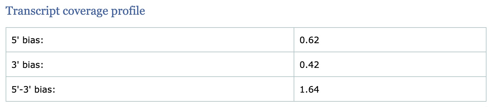
Answer
The 5’-3’ bias measures the ratio of read coverage at the 5’ end versus the 3’ end of transcripts. In an ideal library, coverage should be uniform across the transcript body (ratio ~1). Significant 3’ bias (ratio <1) often indicates: (1) RNA degradation before library preparation (degraded RNA loses 5’ ends first), (2) Poly-A selection bias (primers start from 3’ poly-A tail), or (3) Oligo-dT priming issues. Significant 5’ bias is less common but can occur with certain library preparation methods. This metric is crucial for assessing RNA quality and whether samples are comparable.
Why is it important to check the percentage of reads mapping to exonic, intronic, and intergenic regions in RNA-seq?
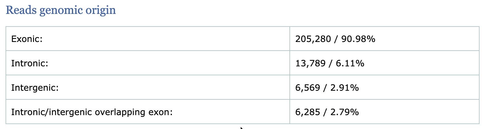
Answer
The distribution of reads across genomic features provides quality insights: (1) High exonic percentage (>70-80%) indicates successful mRNA enrichment, (2) High intronic percentage may indicate genomic DNA contamination, incomplete splicing (nascent transcripts), or nuclear RNA, (3) High intergenic percentage suggests DNA contamination, poor annotation, or novel transcripts. The expected distribution depends on the library type - poly-A selection should show high exonic rates, while total RNA libraries will have more intronic reads. Significant deviations from expected patterns may indicate sample or library preparation issues.
How would you interpret a QualiMap report showing highly variable gene body coverage (non-uniform coverage across transcript length)?
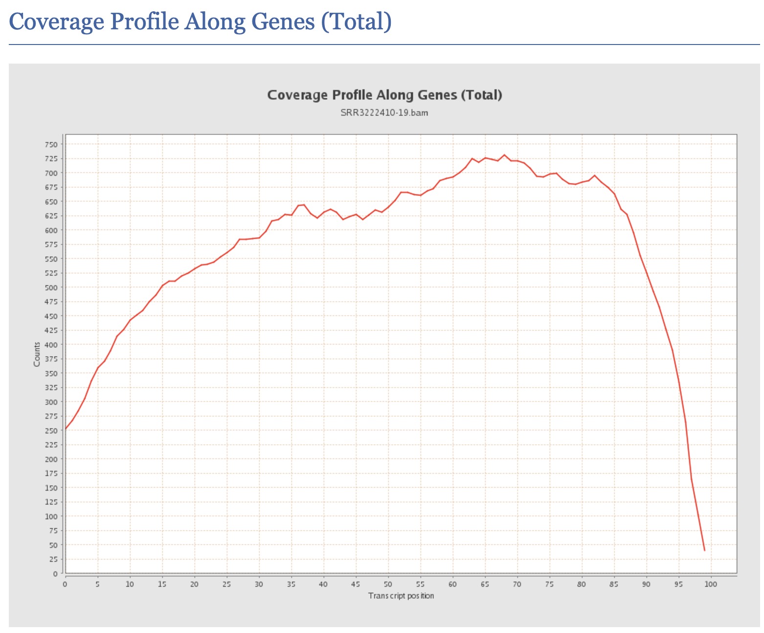
Answer
Non-uniform gene body coverage can indicate: (1) RNA degradation - typically shows 3’ bias with dropout at 5’ ends, (2) Fragmentation bias - certain fragmentation methods have sequence preferences, (3) GC bias - extreme GC regions may have different coverage, (4) Library complexity issues - low complexity libraries may show uneven coverage, (5) Amplification bias - PCR can preferentially amplify certain fragments. To address this: check RNA Integrity Number (RIN) from original QC, compare across samples for systematic effects, and consider using tools that model coverage bias during quantification (like Salmon or RSEM).
What does the QualiMap “junction analysis” section report, and how can it help assess the quality of a splice-aware alignment?
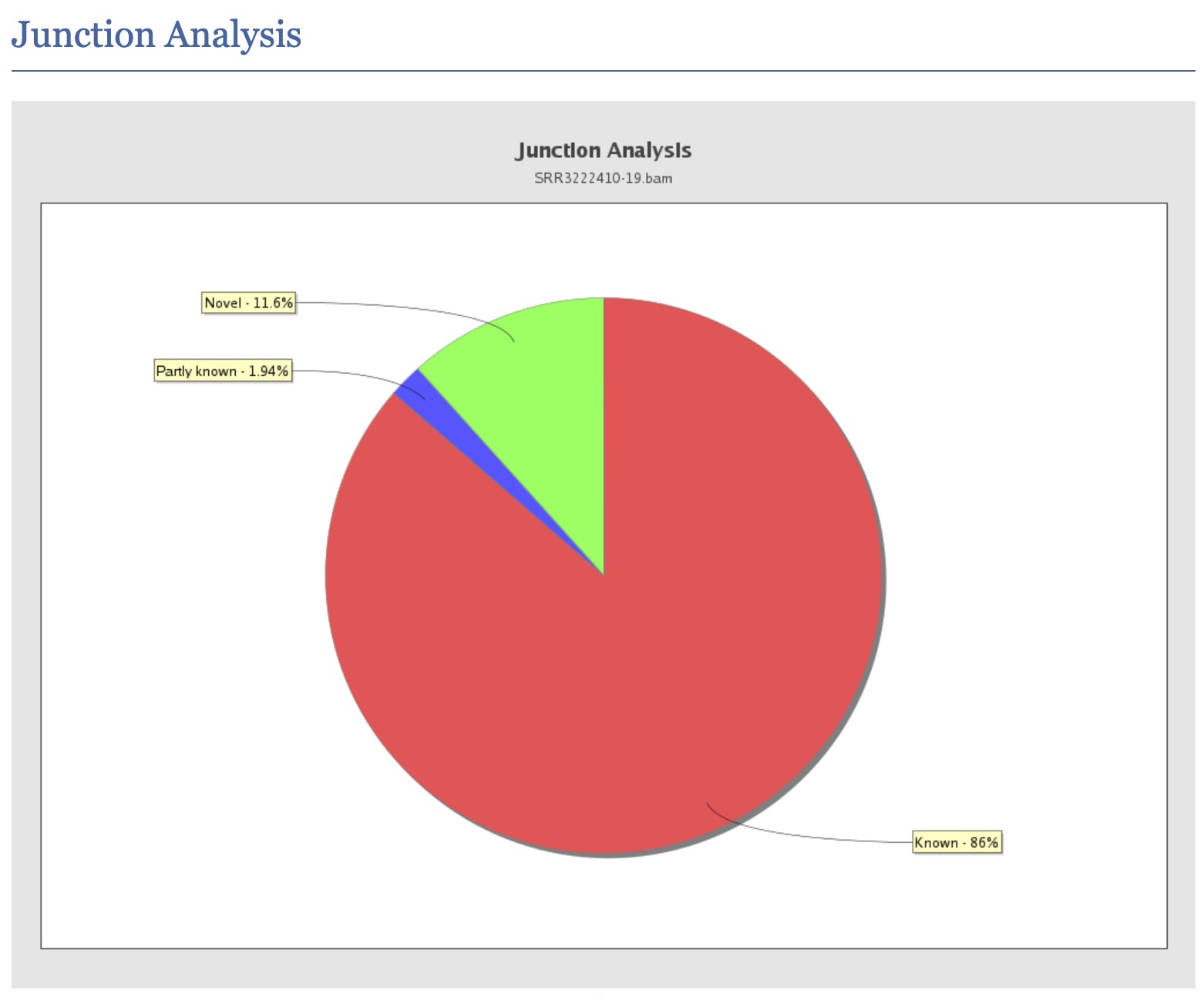
Answer
The junction analysis section reports statistics on reads that span splice junctions, including: (1) Known junctions - reads whose splice sites match annotated exon-exon junctions in the GTF/GFF file, (2) Novel junctions - reads spanning splice sites not present in the annotation, which may represent novel isoforms or mis-splicing events, (3) Partial novel junctions - one splice site is known but the other is not. For a high-quality alignment: a large fraction of junction reads should map to known junctions (typically >80-90% for well-annotated organisms), a very high rate of novel junctions can indicate misalignment, incorrect annotation, or genuine alternative splicing in the sample. This section also helps verify that a splice-aware aligner (e.g., STAR, HISAT2) was used correctly, as an unsplice-aware aligner would produce very few junction-spanning reads.
QualiMap shows your sample has 95% of reads within exons but very low “reads mapped to genes”. What could explain this discrepancy?
Answer
This discrepancy could arise from: (1) Annotation mismatch - using a GTF file from a different genome version or source than the reference FASTA, causing coordinate misalignment, (2) Chromosome naming inconsistency - the BAM file uses “chr1” while GTF uses “1” or vice versa, (3) Feature type specification - the tool may be counting only specific feature types (e.g., protein-coding genes) while reads map to other annotated exons (pseudogenes, lncRNAs), (4) Strand specificity settings - if strand-specific counting is specified but the library is unstranded, many reads may be discarded. Always verify that reference genome, annotation, and counting parameters are consistent.
3.5 Quantification
Counting mapped reads using featureCounts
After ensuring mapping quality, we can move on to enumerating reads mapping to genomic features of interest. Here we will use featureCounts, an ultrafast and accurate read summarization program, that can count mapped reads for genomic features such as genes, exons, promoter, gene bodies, genomic bins and chromosomal locations.
Read featureCounts documentation and see if you can figure it out how to use paired-end reads using an unstranded library to count fragments overlapping with exonic regions and summarise over genes.
Load the subread module on HPC. Create a bash script named featurecounts.sh in the directory scripts.
We could run featureCounts on each BAM file, produce a text output for each sample and combine the output. But the easier way is to provide a list of all BAM files and featureCounts will combine counts for all samples into one text file.
Below is the script that we will use:
#!/bin/bash

# load modules
module load PDC/24.11
module load R/4.4.2-cpeGNU-24.11
module load subread/2.1.1

featureCounts \
  -a "../reference/Mus_musculus.GRCm38.99.gtf" \
  -o "counts.txt" \
  -F "GTF" \
  -t "exon" \
  -g "gene_id" \
  -p \
  -s 0 \
  -T 1 \
  ../3_mapping/*.bam
In the above script, we indicate the path of the annotation file (-a "../reference/Mus_musculus.GRCm38.99.gtf"), specify the output file name (-o "counts.txt"), specify that that annotation file is in GTF format (-F "GTF"), specify that reads are to be counted over exonic features (-t "exon") and summarised to the gene level (-g "gene_id"). We also specify that the reads are paired-end (-p), the library is unstranded (-s 0) and the number of threads to use (-T 1).
Run the featurecounts bash script in the directory 5_dge. Use pwd to check if you are standing in the correct directory.
You should be standing here to run this:
/cfs/klemming/projects/supr/naiss2026-4-45/username/rnaseq/5_dgebash ../scripts/featurecounts.shYou should have two output files:
ls -l-rw-rw-r-- 1 user gXXXXXXX 2.8M Sep 15 11:05 counts.txt
-rw-rw-r-- 1 user gXXXXXXX 658 Sep 15 11:05 counts.txt.summaryInspect the files and try to make sense of them.
3.5.1 Questions
- What is the difference between counting at the exon level versus the gene level, and when might you choose one over the other?
Answer
Gene-level counting sums all reads mapping to any exon of a gene, providing a single expression value per gene. This is simpler and most common for standard DGE analysis. Exon-level counting provides separate counts for each exon, which is useful for: (1) Differential exon usage analysis (detecting alternative splicing), (2) Identifying transcript isoform changes, (3) Detecting exon-skipping events. Gene-level counting is preferred when you’re interested in overall gene expression changes, while exon-level counting is necessary when investigating splicing regulation or isoform-specific expression. Tools like DEXSeq use exon-level counts to identify differential exon usage.
Why does featureCounts need to know if the library is stranded, and what happens if you specify the wrong strandedness?
Answer
Library strandedness indicates whether the sequenced reads preserve the original RNA strand orientation. With
-s 0(unstranded), reads are counted regardless of which strand they map to. With-s 1(stranded) or-s 2(reverse-stranded), only reads matching the expected strand orientation are counted. If you specify stranded counting on an unstranded library: ~50% of reads will be discarded, reducing counts dramatically. If you specify unstranded on a stranded library: you’ll lose strand information and may incorrectly count reads from overlapping genes on opposite strands, creating spurious expression signals. Always verify strandedness using tools like RSeQC’sinfer_experiment.pybefore counting.What does the featureCounts summary file tell you about “Unassigned_Ambiguity” and why might high ambiguity be problematic?
Answer
“Unassigned_Ambiguity” indicates reads that overlap multiple features (genes) and cannot be uniquely assigned. High ambiguity (>10-15%) may indicate: (1) Overlapping gene annotations (common in compact genomes or with comprehensive annotations including antisense transcripts), (2) Using inappropriate counting parameters for your annotation, (3) High rate of multi-gene read-through transcription. This is problematic because ambiguous reads are typically discarded, reducing effective library size and potentially biasing results against genes in crowded genomic regions. Solutions include using different overlap resolution modes (e.g., fractional counting) or annotation filtering.
How does paired-end counting differ from single-end, and what does the
-pflag do in featureCounts?Answer
With the
-pflag, featureCounts counts fragments (the original RNA molecule) rather than individual reads. Both reads of a pair are considered together, and only one count is added if both reads map to the same gene. This is important because: (1) It avoids double-counting the same RNA fragment, (2) It can use the pairing information to resolve ambiguous assignments (if one read is ambiguous but its mate is unique), (3) Fragment counts better represent the number of original RNA molecules. Without-p, each read is counted independently, potentially inflating counts. Additional flags like--countReadPairsand-C(don’t count discordant pairs) refine paired-end behavior.Why might you choose alignment-free quantification methods (Salmon, kallisto) over traditional alignment-based counting (HISAT2 + featureCounts)?
Answer
Alignment-free (pseudoalignment) methods offer several advantages: (1) Speed - 10-100x faster as they don’t compute full alignments, (2) Lower memory requirements, (3) Direct transcript-level quantification with proper handling of multi-mapping reads using expectation-maximization, (4) Better handling of reads from gene families and duplicated regions, (5) Built-in bias correction models (GC bias, sequence bias, positional bias). However, alignment-based methods are preferred when: (1) You need BAM files for visualization or variant calling, (2) You’re working with novel/unannotated transcripts, (3) You’re studying splicing using reads spanning junctions. Many modern pipelines (like nf-core/rnaseq) use STAR for alignment (providing BAMs) and Salmon for quantification.
Important
For downstream steps, we will NOT use this counts.txt file. Instead we will use counts_full.txt from the back-up folder. This contains counts across all chromosomes which will be a better representation of the data for downstream analysis.
The counts_full.txt file is located here: /sw/courses/ngsintro/rnaseq/dardel/main/5_dge/. Copy this file to your 5_dge directory. Remember to replace username.
cp /sw/courses/ngsintro/rnaseq/dardel/main/5_dge/counts_full.txt /cfs/klemming/projects/supr/naiss2026-4-45/username/rnaseq/5_dge/3.6 QC report
Combined QC report using MultiQC
We will use the tool MultiQC to crawl through the output, log files etc from FastQC, HISAT2, QualiMap and featureCounts to create a combined QC report.
Move to the 6_multiqc directory. You should be standing here to run this:
/cfs/klemming/projects/supr/naiss2026-4-45/username/rnaseq/6_multiqcAnd run this in the terminal.
module load PDC/24.11
module load multiqc/1.30

multiqc --interactive ../
/// MultiQC 🔍 | v1.12
| multiqc | Search path : /cfs/klemming/home/r/user/ngsintro/rnaseq
| searching | ━━━━━━━━━━━━━━━━━━━━━━━━━━━━━━━━━━━━━━━━ 100% 297/297
| qualimap | Found 6 RNASeq reports
| feature_counts | Found 6 reports
| bowtie2 | Found 6 reports
| fastqc | Found 12 reports
| multiqc | Compressing plot data
| multiqc | Report : multiqc_report.html
| multiqc | Data : multiqc_data
| multiqc | MultiQC completeThe output should look like below:
ls -ldrwxrwsr-x 2 user gXXXXXXX 4.0K Sep 6 22:33 multiqc_data
-rw-rw-r-- 1 user gXXXXXXX 1.3M Sep 6 22:33 multiqc_report.html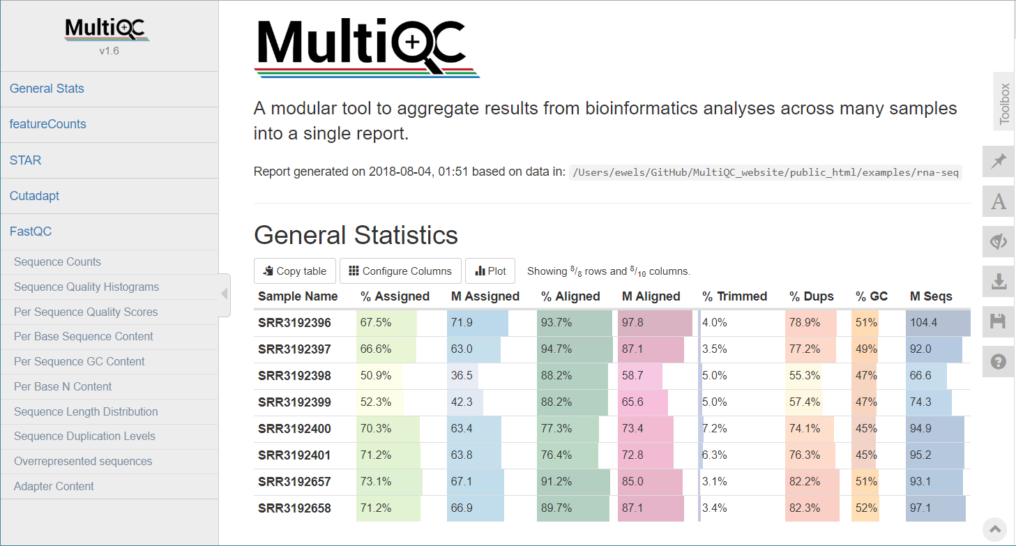
Download the MultiQC HTML report to your computer and inspect the report.
Run this step in a LOCAL terminal and NOT on HPC. Remember to replace username.
scp username@dardel.pdc.kth.se:/cfs/klemming/projects/supr/naiss2026-4-45/username/rnaseq/6_multiqc/multiqc_report.html .3.7 DGE
Differential gene expression using DESeq2
The easiest way to perform differential expression is to use one of the statistical packages, within R environment, that were specifically designed for analyses of read counts arising from RNA-seq, SAGE and similar technologies. Here, we will use one such package called DESeq2. Learning R is beyond the scope of this course so we prepared basic ready to run R scripts to find DE genes between conditions KO and Wt.
We need some annotation information, so we will copy this file /sw/courses/ngsintro/rnaseq/dardel/main/reference/mm-biomart99-genes.txt.gz to your rnaseq/reference directory. Remember to replace username.
cp /sw/courses/ngsintro/rnaseq/dardel/main/reference/mm-biomart99-genes.txt.gz /cfs/klemming/projects/supr/naiss2026-4-45/username/rnaseq/reference/Then decompress the file. gunzip ../reference/mm-biomart99-genes.txt.gz
Move to the 5_dge directory and load R module for use.
module unload qualimap/2.3 # if qualimap was loaded before
module load PDC/24.11
module load R/4.4.2-cpeGNU-24.11
Use pwd to check if you are standing in the correct directory.
Make sure you have the counts_full.txt. If not, you can copy this file: /sw/courses/ngsintro/rnaseq/dardel/main/5_dge/counts_full.txt to your 5_dge directory.
cp /sw/courses/ngsintro/rnaseq/dardel/main/5_dge/counts_full.txt .Copy the DGE R script to your scripts directory and run it.
cp /sw/courses/ngsintro/rnaseq/dardel/main/scripts/dge.r ../scripts/
Rscript ../scripts/dge.r
If you are curious what’s inside dge.r, you are welcome to explore it using a text editor. Very briefly, the steps are as follows:
Prepare the metadata table which contains sample information (sample name, condition, batch etc). This is required for DESeq2 to perform the analysis. In this case, we have two conditions (KO and Wt) and three replicates for each condition.
Read in the counts file and prepare the count matrix. The count matrix should have genes as rows and samples as columns. Make sure that the order of samples in the count matrix matches the order of samples in the metadata table.
Filter out lowly expressed genes. This step can help improve the power of the analysis by removing genes that are not expressed or have very low counts across all samples. A common threshold is to keep genes that have at least n counts in at least 3 samples (in at least one condition).
Create a DESeqDataSet object using the count matrix and metadata table. Size factors are estimated to account for differences in sequencing depth between samples. Dispersions are estimated to model the variance in the data, which is crucial for accurate DGE testing. Wald test is performed to identify differentially expressed genes between the conditions. Contrasts are specified to compare KO vs Wt.
We have the following line:
res <- results(dg, contrast = c("condition", "KO", "Wt"), alpha = 0.05)which is the line that performs the actual DGE testing. The
contrastargument specifies the comparison we want to make (KO vs Wt) andalphaspecifies the significance threshold for adjusted p-value. The order of the conditions in the contrast matters. In this case, positive log2 fold-change values will indicate genes overexpressed in KO compared to Wt, while negative values are vice versa.Gene annotation information is added to the results using the biomart file we downloaded earlier. This step is optional but can help with interpretation of results.
Variance stabilising transformation (VST) is applied to the count data to produce a matrix of normalised counts that can be used for exploratory analyses like PCA and clustering. VST helps to stabilise the variance across the range of mean values, making it easier to visualize and interpret patterns in the data.
This should have produced the following output files:
ls -l-rw-rw-r-- 1 user gXXXXXXX 282K Jan 22 23:16 counts_vst_full.rds
-rw-rw-r-- 1 user gXXXXXXX 1.7M Jan 22 23:16 counts_vst_full.txt
-rw-rw-r-- 1 user gXXXXXXX 727K Jan 22 23:16 dge_results_full.rds
-rw-rw-r-- 1 user gXXXXXXX 1.7M Jan 22 23:16 dge_results_full.txtEssentially, we have two outputs: dge_results_full and counts_vst_full. dge_results_full is the list of differentially expressed genes. This is available in human readable tab-delimited .txt file and R readable binary .rds file. The counts_vst_full is variance-stabilised normalised counts, useful for exploratory analyses.
ensembl_gene_id baseMean    log2FoldChange  lfcSE   stat    pvalue  padj
ENSMUSG00000000001  4759.98141172752    -0.22313384713415   0.0980746249168413  -2.27512354454562   0.0228985196324456  0.119582057119404
ENSMUSG00000000028  301.589906387388    0.165180329556362   0.189505963839622   0.871635496115001   0.383407259765523   0.697400109793806
ENSMUSG00000000031  67354.9059955111    0.485425313069624   0.117601047180511   4.12773347973738    3.66356379521764e-05    0.000585338479238071
Copy the results text file (dge_results_full.txt) to your computer and inspect the results. What are the columns? How many differentially expressed genes are present after adjusted p-value of 0.05? How many genes are upregulated and how many are down-regulated? How does this change if we set a log2 fold-change cut-off of ±1?
Open in a spreadsheet editor like Microsoft Excel or LibreOffice Calc.
If you do not have the results or were unable to run the DGE step, you can copy these two here which will be required for functional annotation (optional).
cp /sw/courses/ngsintro/rnaseq/dardel/main/5_dge/dge_results_full.txt .
cp /sw/courses/ngsintro/rnaseq/dardel/main/5_dge/dge_results_full.rds .
cp /sw/courses/ngsintro/rnaseq/dardel/main/5_dge/counts_vst_full.txt .
cp /sw/courses/ngsintro/rnaseq/dardel/main/5_dge/counts_vst_full.rds .
3.7.1 Questions
Why does DESeq2 use raw counts instead of normalized counts (like TPM or FPKM) as input?
Answer
DESeq2 uses raw counts because it needs the integer count data to model the variance structure using a negative binomial distribution. Pre-normalized values (TPM, FPKM) have already had variance-altering transformations applied, which would violate the statistical model’s assumptions. DESeq2 performs its own normalization internally using size factors that account for library size and composition differences. Using raw counts allows DESeq2 to properly estimate dispersion parameters and perform accurate statistical tests.
What is the purpose of the adjusted p-value (padj) in DESeq2 results, and why is it different from the raw p-value?
Answer
The adjusted p-value corrects for multiple hypothesis testing. When testing thousands of genes, even with a significance threshold of 0.05, we’d expect ~5% false positives by chance alone (e.g., 500 false positives when testing 10,000 genes). DESeq2 uses the Benjamini-Hochberg procedure to control the False Discovery Rate (FDR). The adjusted p-value represents the expected proportion of false positives among all genes called significant at that threshold. For example, padj < 0.05 means we expect fewer than 5% of the significant calls to be false positives, making it a more reliable measure for identifying truly differentially expressed genes.
Why might some genes have NA values for padj in DESeq2 results?
Answer
DESeq2 assigns NA to padj for several reasons: (1) Genes with zero counts across all samples - no data to analyze, (2) Genes with only a single sample having a nonzero count - insufficient data for statistical testing, (3) Genes with extreme count outliers that fail DESeq2’s outlier detection (Cook’s distance), (4) Genes automatically filtered due to low counts (independent filtering) to increase power for remaining tests. These NAs are intentional and help focus analysis on genes with sufficient evidence for reliable statistical testing. You can use
results(dds, cooksCutoff=FALSE)to disable outlier filtering if needed.What biological interpretation can you draw from a gene with high baseMean but low log2FoldChange versus a gene with low baseMean but high log2FoldChange?
Answer
A gene with high baseMean but low log2FoldChange is highly expressed but changes only slightly between conditions - potentially a constitutively expressed gene with minor condition-specific modulation (e.g., a housekeeping gene responding to stress). A gene with low baseMean but high log2FoldChange shows dramatic expression changes but at low absolute levels - this could be a regulatory gene (transcription factors often have low expression but large fold changes) or a condition-specific marker. However, lowly expressed genes with high fold changes should be interpreted with caution, as they may be more susceptible to noise and have less reliable statistical estimates. Always consider both fold change and expression level when interpreting biological significance.
In the context of this experiment (YAP/TAZ knockout in Schwann cells), what would you expect to see in terms of direction of change for myelination-related genes?
Answer
Since YAP and TAZ are transcriptional co-activators that promote cell proliferation and are essential for myelination, their knockout would be expected to: (1) Downregulate genes involved in myelin sheath formation (e.g., Mbp, Mpz, Pmp22), (2) Downregulate lipid biosynthesis genes essential for myelin membrane (myelin is ~70% lipid), (3) Potentially upregulate apoptosis-related genes (Hippo pathway normally inhibits apoptosis), (4) Alter cell cycle genes since YAP/TAZ promote proliferation, (5) Change expression of laminin receptor genes as mentioned in the paper title. Comparing your DE gene list to known myelination pathways would validate the experimental system.
3.8 RNA-Seq plots
We use R to create exploratory plots and investigate the results of differential expression analysis. Depending on your proficiency in reading R code and using R, you can in this section either just call scripts from the command lines with a set of arguments or you can open the R script in a text editor, and run the code step by step from an interactive R session.
Load the module R.
module load PDC/24.11
module load R/4.4.2-cpeGNU-24.11
3.8.1 PCA plot
A popular way to visualise general patterns of gene expression in your data is to produce either PCA (Principal Component Analysis) or MDS (Multi Dimensional Scaling) plots. These methods aim at summarising the main patterns of expression in the data and display them on a two-dimensional space and still retain as much information as possible. To properly evaluate these kind of results is non-trivial, but in the case of RNA-seq data we often use them to get an idea of the difference in expression between treatments and also to get an idea of the similarity among replicates. If the plots shows clear clusters of samples that corresponds to treatment it is an indication of treatment actually having an effect on gene expression. If the distance between replicates from a single treatment is very large it suggests large variance within the treatment, something that will influence the detection of differentially expressed genes between treatments.
Move to the 5_dge/ directory. Then copy and run the pca.r script like below.
cp /sw/courses/ngsintro/rnaseq/dardel/main/scripts/pca.r ../scripts/
Rscript ../scripts/pca.r
This generates a file named pca.png in the 5_dge folder. To view it, download it to your local disk.
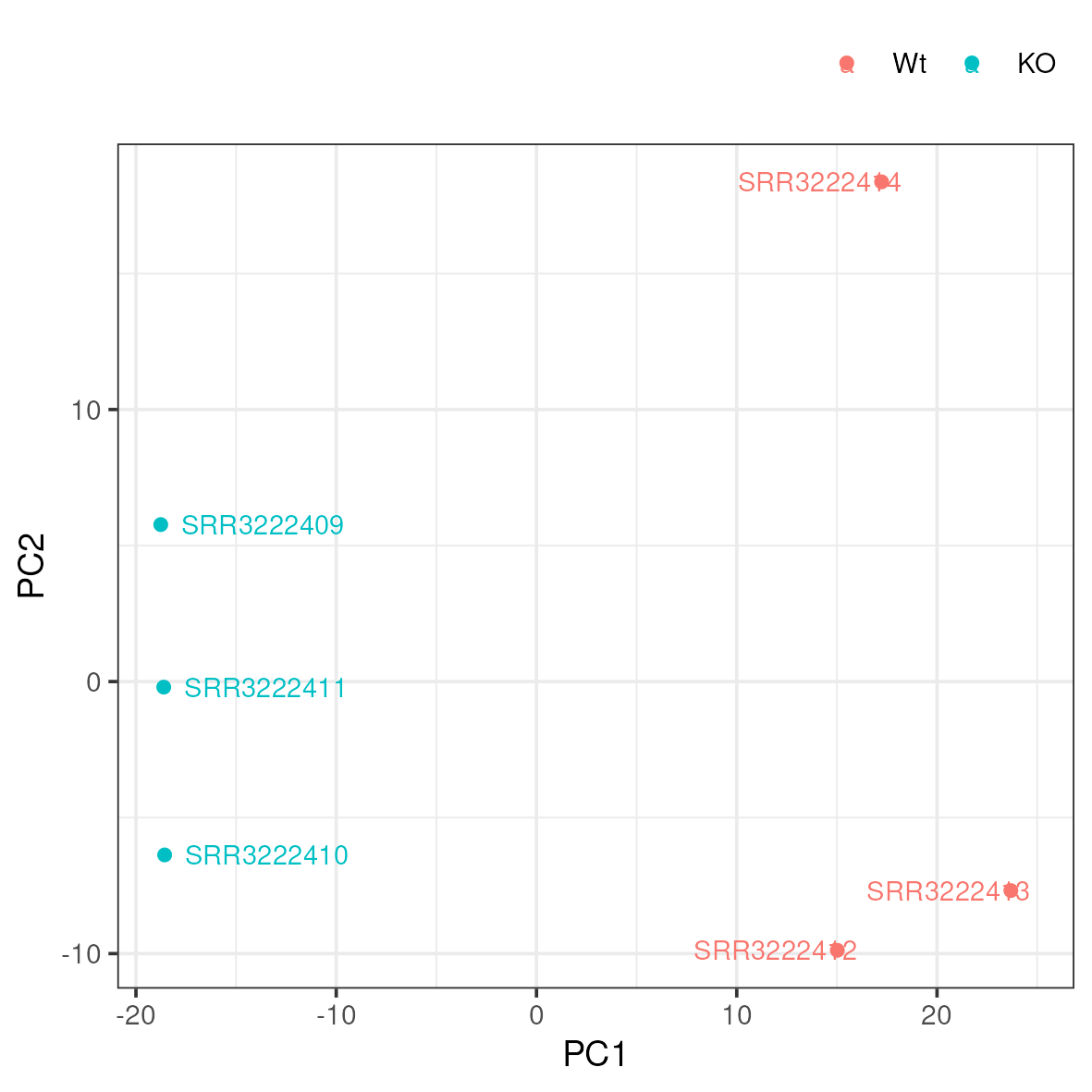
Do samples cluster as expected? Are there any odd or mislabelled samples? Based on these results, would you expect to find a large number of significant DE genes?
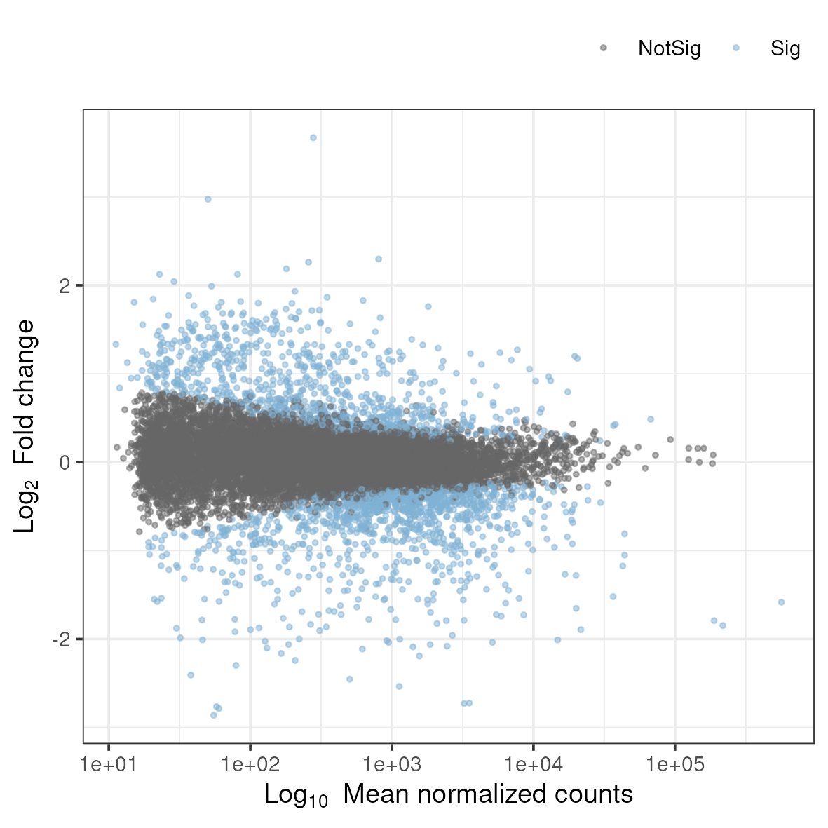
3.8.2 MA plot
An MA-plot plots the mean expression and estimated log-fold-change for all genes in an analysis.
Copy and run the ma.r script in the 5_dge directory.
cp /sw/courses/ngsintro/rnaseq/dardel/main/scripts/ma.r ../scripts/
Rscript ../scripts/ma.r
This generates a file named ma.png in the 5_dge folder. To view it, download it to your local disk.
3.8.3 Volcano plot
A related type of figure will instead plot fold change (on log2 scale) on the x-axis and -log10 p-value on the y-axis. Scaling like this means that genes with lowest p-value will be found at the top of the plot.
Copy and run the script named volcano.r in the 5_dge directory.
cp /sw/courses/ngsintro/rnaseq/dardel/main/scripts/volcano.r ../scripts/
Rscript ../scripts/volcano.r
This generates a file named volcano.png in the 5_dge folder. To view it, download it to your local disk.
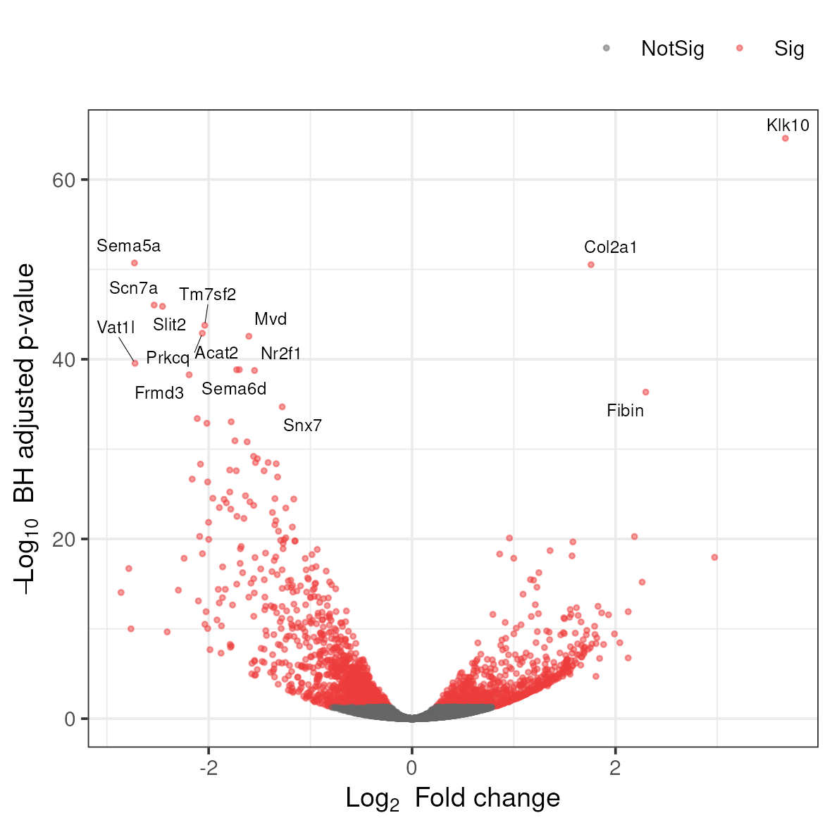
Anything noteworthy about the patterns in the plot? What do you think are the different colors? Is there a general trend in the direction of change in gene expression as a consequence of the experiment?
3.8.4 Heatmap
Another popular plots for genome-wide expression patterns is heatmap for a set of genes. If you run the script called heatmap.r, it will extract the top 50 genes that have the lowest p-value in the experiment and create a heatmap from these. In addition to color-coding the expression levels over samples for the genes it also clusters the samples and genes based on inferred distance between them.
Run the script named heatmap.r in the 5_dge directory.
cp /sw/courses/ngsintro/rnaseq/dardel/main/scripts/heatmap.r ../scripts/
Rscript ../scripts/heatmap.r
This generates a file named heatmap.png in the 5_dge folder. To view it, download it to your local disk.
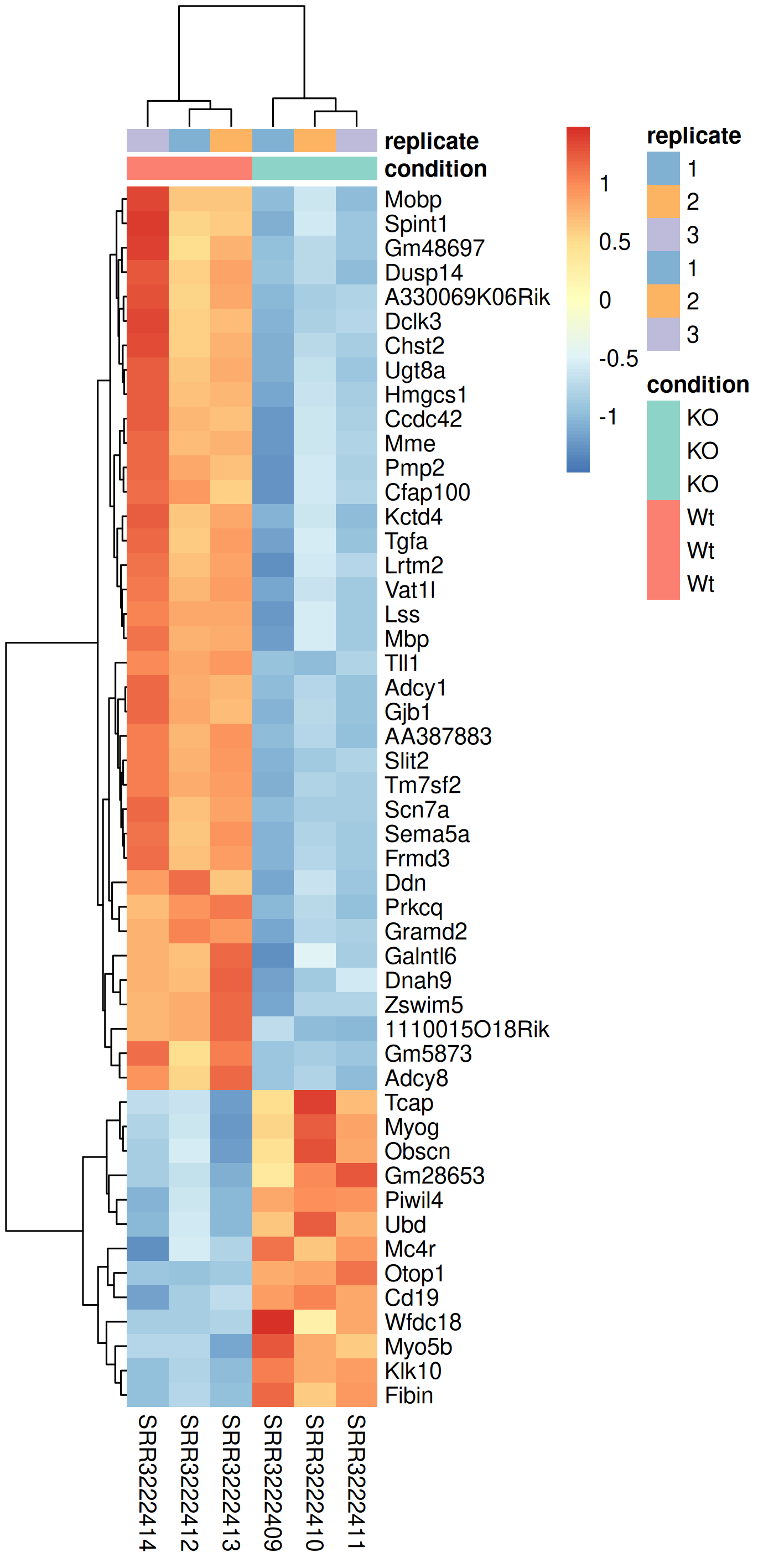
Compare this plot to a similar plot in the paper behind the data.
3.8.5 Questions
In a PCA plot, what does it mean biologically if PC1 explains 80% of the variance and separates your treatment groups perfectly?
Answer
This indicates that the experimental treatment (e.g., gene knockout) is the dominant source of variation in the dataset, which is ideal. It means: (1) The treatment has a strong, consistent effect on gene expression, (2) Technical variation and batch effects are relatively minor compared to the biological effect, (3) Replicates within each group are similar to each other, (4) You should have good statistical power to detect DE genes. However, if PC1 doesn’t separate treatment groups but PC2 or PC3 does, there may be unwanted technical variation (batch effects) that should be addressed. If treatment groups don’t separate on any major PC, the effect may be subtle or absent.
Why does the MA plot show a funnel shape, with more spread at lower expression levels?
Answer
This pattern reflects the statistical properties of count data. At low expression levels: (1) Poisson counting noise is relatively large compared to the signal (coefficient of variation is higher), (2) A difference of a few counts represents a large fold-change but may not be statistically reliable, (3) Biological variation is harder to estimate accurately. At high expression levels, the relative noise decreases, and fold-change estimates become more precise. This is why DESeq2 and other tools apply shrinkage to log2FoldChange estimates - to reduce the artificially inflated fold-changes for lowly expressed genes. The MA plot helps visualize whether appropriate shrinkage has been applied.
What does it mean if your volcano plot shows more significantly underexpressed genes than overexpressed genes?
Answer
An asymmetric volcano plot suggests a directional effect of the experimental treatment. In the context of YAP/TAZ knockout: since YAP/TAZ are transcriptional co-activators, knocking them out should predominantly reduce the expression of their target genes, leading to more underexpressed genes. However, indirect effects through regulatory cascades can cause upregulation of other genes (e.g., genes normally repressed by YAP/TAZ targets). The asymmetry can provide biological insight about whether your perturbation mainly activates or represses transcription. You should verify this pattern is reproducible and not due to technical artifacts like RNA quality differences between conditions.
In a heatmap of DE genes, why might samples from the same treatment group not cluster perfectly together?
Answer
Imperfect clustering within treatment groups can occur due to: (1) Biological variability between replicates (individual animals, genetic background variation), (2) Batch effects if samples were processed on different days, (3) Sample quality differences (RNA integrity, library complexity), (4) Outlier samples that should potentially be removed, (5) The subset of genes shown may not fully represent the treatment effect (only top 50 genes shown). This is why it’s important to look at PCA first (uses all genes) before interpreting heatmaps of selected genes. If one replicate consistently appears as an outlier across multiple analyses, consider investigating sample quality or potential mislabeling.
How would you decide whether to use z-score normalization (row scaling) versus showing absolute expression values in a heatmap?
Answer
Z-score normalization (scaling each gene to mean=0, SD=1) is preferred when: (1) You want to compare relative changes across genes with very different expression levels, (2) The focus is on expression patterns rather than absolute levels, (3) Genes with high expression would otherwise dominate the color scale. Absolute values are better when: (1) You want to see which genes are highly versus lowly expressed, (2) Comparing magnitude of expression between genes is meaningful, (3) You’re interested in co-expression of genes at similar absolute levels. Most differential expression heatmaps use z-scores because DE genes span a wide expression range, and the biological question is usually about patterns of change rather than absolute expression.
4 Bonus exercises
Optional
These exercises are optional and to be run only if you have time and you want to explore this topic further.
4.1 Gene set analysis
In this part of the exercise, we will try some approaches to make sense of the differentially expressed genes. If you are not closely familiar with the genes and it’s relationship to your experimental setup, it’s hard to draw conclusions by simply looking at the gene list. We will use gene set analysis (GSA) and gene set enrichment analysis (GSEA) that ingests the gene list and returns to us functional terms which may be more meaningful in understanding the biological consequences of your experiment. We will use Gene Ontology (GO) database.
When performing this type of analysis, one has to keep in mind that the analysis is only as accurate as the annotation available for your organism. So, if working with non-model organisms which do have experimentally-validated annotations (computationally inferred), the results may not be fully reflecting the actual situation.
There are many methods to approach the question as to which biological processes and pathways are over-represented amongst the differentially expressed genes, compared to all the genes included in the DE analysis. They use several types of statistical tests (e.g. hypergeometric test, Fisher’s exact test etc.), and many have been developed with microarray data in mind.
We will use the R / Bioconductor package clusterProfiler. This package provides methods for performing gene set analysis and gene set enrichment analysis.
In this part, we will use the same data as in the main workflow. The starting point of the exercise is the file with results of the differential expression produced in the main part of the exercise.
Change to the 5_dge directory in your rnaseq directory.
cd 5_dgeLoad R module
module load PDC/24.11
module load R/4.4.2-cpeGNU-24.11
Copy and run the GSE script from the linux terminal.
cp /sw/courses/ngsintro/rnaseq/dardel/main/scripts/gse-clusterprofiler.r ../scripts/
Rscript ../scripts/gse-clusterprofiler.r
It will read the dge_results_full.rds and filter the table to get the differentially expressed genes and perform over-representation analysis. When completed, you should find the following files:
ls -l-rw-r--r-- 1 user staff 3.8M Jan 4 16:00 gse-bp.rds
-rw-r--r-- 1 user staff 205K Jan 4 16:00 gse-bp.txt
-rw-r--r-- 1 user staff 1.0M Jan 4 16:00 gse-cc.rds
-rw-r--r-- 1 user staff 31K Jan 4 16:00 gse-cc.txt
-rw-r--r-- 1 user staff 841K Jan 4 16:00 gse-mf.rds
-rw-r--r-- 1 user staff 14K Jan 4 16:00 gse-mf.txtThe results are GO terms from three different gene ontology databases: Biological process (BP), cellular component (CC) and molecular function (MF). They are written as text files and RDS files which is an R specific format.
ID  Description GeneRatio   BgRatio RichFactor  FoldEnrichment  zScore  pvalue  p.adjust    qvalue  geneID  Count
GO:0051146  striated muscle cell differentiation    108/1845    284/11989   0.380281690140845   2.47110958433528    10.7000404150557    4.12598986480192e-21    1.94178291659553e-17    1.60695883528152e-17    Ccnd2/Rpl3l...  108
GO:0003012  muscle system process   124/1845    351/11989   0.353276353276353   2.29562612435241    10.5065712553733    7.18912594074615e-21    1.94178291659553e-17    1.60695883528152e-17    Tbx2/Scn4a...   124
Take a quick look at some of these files.
head gse-bp.txt | cut -f2Description
striated muscle cell differentiation
muscle system process
cellular component assembly involved in morphogenesis
muscle tissue development
muscle contraction
muscle organ development
muscle cell development
striated muscle cell development
muscle cell differentiationhead gse-cc.txt | cut -f2Description
myofibril
sarcomere
contractile fiber
I band
Z disc
striated muscle thin filament
myofilament
actin cytoskeleton
synaptic membraneExplore the output files and figure out what the columns mean. Do you think the terms reflects the biology of the experiment we have just analysed?
4.1.1 Questions
What is the difference between gene set over-representation analysis (ORA) and gene set enrichment analysis (GSEA)?
Answer
Over-representation analysis (ORA) takes a pre-defined list of DE genes (based on p-value and fold-change cutoffs) and tests whether certain pathways have more genes than expected by chance using a hypergeometric test. GSEA, in contrast, uses the entire ranked gene list (typically by fold-change or a combined statistic) without applying arbitrary cutoffs, and tests whether genes in a pathway tend to cluster toward the top or bottom of the ranked list. GSEA can detect coordinated changes in a pathway even when individual genes don’t pass significance thresholds. ORA is simpler and faster but can miss subtle, coordinated pathway changes; GSEA is more sensitive to pathway-level effects but requires a meaningful ranking metric.
What does the “GeneRatio” column in enrichment results tell you, and why might two terms with the same p-value have different biological significance?
Answer
Gene ratio represents the proportion of genes in a GO term that are differentially expressed (e.g., 15/100 means 15 of 100 genes in that term are DE). Two terms with similar p-values might differ in: (1) Effect size - a term with 50% of genes affected vs. 10% suggests different levels of pathway perturbation, (2) Total term size - enrichment in a large general term (e.g., “metabolic process” with 5000 genes) is less specific than enrichment in a small focused term (e.g., “myelin sheath” with 50 genes), (3) Biological interpretability - some terms are more informative for your specific question. Always consider gene ratio, term size, and biological context together rather than just p-values.
Why is it important to specify an appropriate “background” or “universe” for enrichment analysis?
Answer
The background set defines what genes could have been detected as DE in your experiment. Using the wrong background biases results: (1) If you use all genes in the genome but only measured a subset (e.g., genes on a microarray or genes with detectable expression), you underestimate enrichment, (2) If you use all expressed genes but many have zero counts, you may include genes that could never be detected as DE. The correct background is typically all genes that had sufficient expression to be tested for DE (i.e., genes that passed low-count filtering in DESeq2). Tissue-specific expression patterns also matter - brain-expressed genes are pre-enriched for neural functions, so using whole-genome background inflates neural term enrichment.
How would you interpret enrichment results that show highly redundant GO terms (e.g., “muscle contraction”, “muscle system process”, “striated muscle contraction”)?
Answer
Redundant GO terms arise because: (1) GO is hierarchical - child terms (specific) inherit genes from parent terms (general), (2) The same genes contribute to multiple overlapping terms. To address redundancy: (1) Use semantic similarity methods to cluster related terms (e.g., REVIGO, simplifyEnrichment), (2) Look at the “leading edge” genes - if the same genes drive multiple terms, they represent one biological signal, (3) Focus on the most specific terms that are significant, (4) Use pathway databases with less redundancy (e.g., KEGG, Reactome) alongside GO. ClusterProfiler’s enrichplot functions help visualize term relationships. Reporting cleaned/simplified term lists is better than listing all redundant significant terms.
Why do the GO enrichment results show muscle-related terms when the experiment studies myelination in Schwann cells?
Answer
Read the section ‘A critical reanalysis’ further down.
4.2 IGV browser
Data visualisation is important to be able to clearly convey results, but can also be very helpful as tool for identifying issues and note-worthy patterns in the data. In this part you will use the BAM files you created earlier in the RNA-seq lab and use IGV (Integrated Genomic Viewer) to visualise the mapped reads and genome annotations. In addition we will produce high quality plots of both the mapped read data and the results from differential gene expression.
If you are already familiar with IGV you can load the mouse genome and at least one BAM file from each of the treatments that you created earlier. The functionality of IGV is the same as if you look at genomic data, but there are a few of the features that are more interesting to use for RNA-seq data.
Integrated genomics viewer from Broad Institute is a nice graphical interface to view bam files and genome annotations. It also has tools to export data and some functionality to look at splicing patterns in RNA-seq data sets. Even though it allows for some basic types of analysis it should be used more as a nice way to look at your mapped data. Looking at data in this way might seem like a daunting approach as you can not check more than a few regions, but in in many cases it can reveal mapping patterns that are hard to catch with just summary statistics.
For this tutorial you can chose to run IGV directly on your own computer or on HPC . If you chose to run it on your own computer you will have to download some of the BAM files (and the corresponding index files) from HPC. If you have not yet installed IGV, refer to the pre-course instructions to install it.
Local
Copy two BAM files (one from each experimental group, for example; SRR3222409-19 and SRR3222412-19) and the associated index (.bam.bai) files to your computer by running the below command in a LOCAL terminal and NOT on HPC.
Remember to replace username.
scp username@dardel.pdc.kth.se:/cfs/klemming/projects/supr/naiss2026-4-45/username/rnaseq/3_mapping/SRR3222409-19.bam .
scp username@dardel.pdc.kth.se:/cfs/klemming/projects/supr/naiss2026-4-45/username/rnaseq/3_mapping/SRR3222409-19.bam.bai .
scp username@dardel.pdc.kth.se:/cfs/klemming/projects/supr/naiss2026-4-45/username/rnaseq/3_mapping/SRR3222412-19.bam .
scp username@dardel.pdc.kth.se:/cfs/klemming/projects/supr/naiss2026-4-45/username/rnaseq/3_mapping/SRR3222412-19.bam.bai .
Alternatively, you can use an SFTP browser like Filezilla or Cyberduck for a GUI interface. Windows users can also use the MobaXterm SFTP file browser to drag and drop.
HPC
For Linux and Mac users, Log in to HPC in a way so that the generated graphics are exported via the network to your screen. This will allow any graphical interface that you start on your compute node to be exported to your computer. However, as the graphics are exported over the network, it can be fairly slow in redrawing windows and the experience can be fairly poor.
Login in to HPC with X-forwarding enabled:
ssh -Y username@dardel.pdc.kth.se
ssh -Y computenode
An alternative method is to login through Remote Desktop application: ThinLinc. Once you log into this interface you will have a linux desktop interface in a browser window. This interface is running on the login node, so if you want to do any heavy lifting you need to login to your reserved compute node also here. This is done by opening a terminal in the running linux environment and log on to your compute node as before. If you have no active reservation you have to do that first.
Load necessary modules and start IGV
module load PDC/24.11
module load igv/2.17.4
igv.sh&
This should start the IGV so that it is visible on your screen. If not please try to reconnect to HPC or consider running IGV locally as it provides a better experience.
Once we have the program running, you select the genome that you would like to load. Choose Mouse mm10. Note that if you are working with a genome that are not part of the available genomes in IGV, one can create genome files from within IGV. Please check the manual of IGV for more information on that.
To open your BAM files, go to File > Load from file... and select your BAM file and make sure that you have a .bai index for that BAM file in the same folder. You can repeat this and open multiple BAM files in the same window, which makes it easy to compare samples. Then select Chr19 since we only have data for that one chromosome.
For every file you open a number of panels are opened that visualise the data in different ways. The first panel named Coverage summarises the coverage of base-pairs in the window you have zoomed to. The second panel shows the reads as they are mapped to the genome. If one right click with the mouse on the read panel there many options to group and color reads. The bottom panel named Refseq genes shows the gene models from the annotation.
To see actual reads you have to zoom in until the reads are drawn on screen. If you have a gene of interest you can also use the search box to directly go to that gene.
Here is the list of top 20 differentially expressed genes on Chr19 ordered by absolute fold change. The adjusted p value is shown as padj, the average expression of the gene is shown as baseMean.
   external_gene_name    baseMean log2FoldChange     lfcSE       stat       pvalue         padj
1            AA387883    59.94083      -2.784689 0.2706306  -9.076824 1.117894e-19 1.943690e-17
2              Tm7sf2   947.63388      -2.038574 0.1399445 -14.539498 6.809003e-48 1.677171e-44
3              Ankrd2    59.28633       1.751990 0.2747018   6.323854 2.551188e-10 1.261004e-08
4                Nrap   220.59983       1.699389 0.2680529   6.352080 2.124228e-10 1.067822e-08
5              Slc1a1    63.82987       1.682163 0.2501657   6.651224 2.906652e-11 1.652208e-09
6                Scd1  6678.59981      -1.447372 0.1767165  -8.190325 2.605209e-16 2.961722e-14
7               Fads2  3269.79425      -1.415215 0.1201146 -11.779700 4.966970e-32 3.134559e-29
8             Aldh1a7    65.81205      -1.354443 0.2413361  -5.548387 2.883175e-08 1.002599e-06
9                Lbx1    26.03640       1.335612 0.2954499   4.503693 6.678261e-06 1.328372e-04
10             Ms4a4b    23.27050       1.329984 0.2927615   4.729255 2.253447e-06 5.015617e-05
11             Kcnip2    34.13675      -1.316531 0.2914951  -4.479672 7.475767e-06 1.463369e-04
12               Pygm  1129.47092       1.245257 0.2912826   4.323631 1.534817e-05 2.736196e-04
13              Rbm20    51.36261       1.181655 0.2927293   4.051754 5.083520e-05 7.774718e-04
14            Gm50147    39.53043      -1.179758 0.2754761  -4.239382 2.241359e-05 3.794393e-04
15            Macrod1   244.02353       1.082442 0.1904105   5.681007 1.339039e-08 4.984802e-07
16               Scd2 44054.03491      -1.050473 0.1434332  -7.323814 2.410205e-13 1.874759e-11
17              Fads1  4074.38868      -1.050393 0.1121926  -9.361514 7.860230e-21 1.470460e-18
18             Plaat3  5284.36470      -1.046273 0.1317594  -7.940261 2.017561e-15 2.114719e-13
19              Cd274    35.91671       1.017544 0.2938405   3.474263 5.122580e-04 5.632932e-03
20              Ms4a1    25.80723       1.013036 0.2949268   3.437803 5.864549e-04 6.294275e-03
Have a look at few of the interesting genes on Chr19 using the external_gene_name identifier. Look into gene Tm7sf2 or Ankrd2. You might have to right-click and change option to Squished to see more reads.
Do you expect these genes to be differentially expressed?
To see some genes with large number of reads, see Scd1 or Scd2.
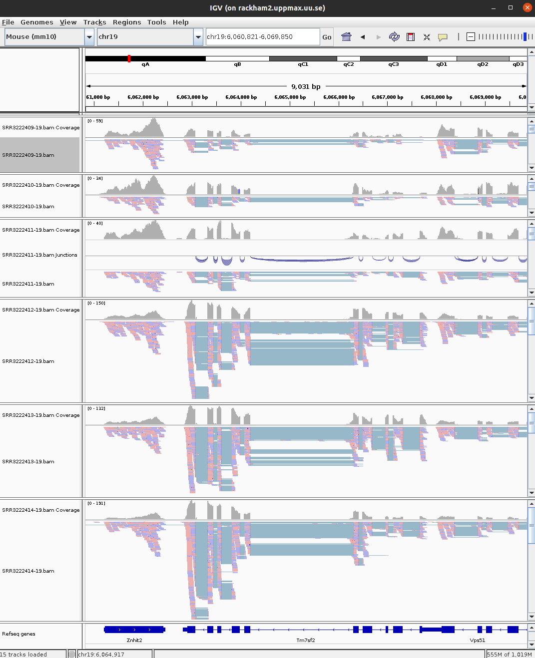
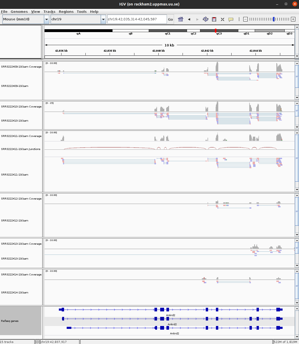
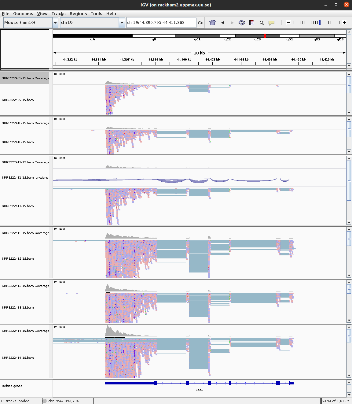
For more detailed information on the splice reads you can instead of just looking at the splice panel right click on the read panel and select Sashimi plots. This will open a new window showing in an easy readable fashion how reads are spliced in mapping and you will also be able to see that there are differences in between what locations reads are spliced. This hence gives some indication on the isoform usage of the gene.
Do you think the reads are from a stranded or unstranded library?
One can visualise all genes in a given pathway using the gene list option under Regions in the menu. If you need hints for how to proceed, see Gene List tutorial at Broad. But, we only have data from one chromosome, so this is not that useful now.
4.2.1 Questions
How can you determine from the IGV visualization whether a gene shows differential expression between conditions?
Answer
In IGV, you can visually assess differential expression by: (1) Comparing the coverage track height between samples from different conditions - higher peaks indicate more reads/expression, (2) Looking at the read density in the read alignment panel, (3) Using IGV’s “Group Autoscale” feature to normalize tracks for fair comparison. However, visual assessment has limitations: it doesn’t account for library size differences, biological variability between replicates, or provide statistical significance. For genes like Tm7sf2 (downregulated in KO), you should see consistently lower coverage across all KO samples compared to Wt samples. IGV is best for qualitative validation of DE results, not for discovering DE genes.
What information can Sashimi plots provide that regular read alignments cannot?
Answer
Sashimi plots specifically visualize splice junctions by showing: (1) Arcs connecting exons that are joined by spliced reads, with numbers indicating how many reads support each junction, (2) Different splice junction usage between samples, revealing alternative splicing, (3) Exon skipping events where reads connect non-adjacent exons, (4) Alternative 5’ or 3’ splice site usage, (5) Novel splice junctions not in the annotation. Regular read alignments show individual reads but make it difficult to quantify junction usage. Sashimi plots aggregate this information, making it easy to compare splicing patterns between conditions and identify isoform switching that might not be detected by gene-level DE analysis.
Why is it important to have a BAM index file (.bai) for visualization in IGV, and what would happen without it?
Answer
BAM index files enable random access to specific genomic regions without reading the entire file. BAM files store reads in coordinate-sorted order, and the index maps genomic positions to file locations. Without an index: (1) IGV cannot quickly jump to a specific gene or region, (2) It would need to scan the entire file sequentially, making navigation extremely slow for large files, (3) Many genome browsers will simply refuse to load unindexed BAM files. The index file contains offset positions at regular intervals, allowing IGV to quickly locate and load only the reads within the current view window. This is essential for interactive visualization of the multi-gigabyte BAM files typical of RNA-seq experiments.
Looking at the read alignments for a gene in IGV, how can you identify potential problems with the sequencing or alignment?
Answer
IGV can reveal several issues: (1) PCR duplicates - many reads with identical start positions, visible as vertical “stacks” (consider using read coloring by duplicate flag), (2) Mapping quality issues - reads colored gray have low mapping quality, indicating multi-mapping, (3) Mismatches - colored bases indicate SNPs, sequencing errors, or misalignment (useful for QC and variant detection), (4) Unusual insert sizes - paired reads too far apart or in wrong orientation indicate structural variants or mapping artifacts, (5) Coverage dropouts within exons - may indicate problematic regions or deletions, (6) High intronic coverage - suggests DNA contamination or unspliced RNA. Color reads by various attributes (strand, pair orientation, insert size) to identify different issues.
How would you use IGV to determine whether the RNA-seq library is stranded, and why does this matter for downstream analysis?
Answer
To check strandedness in IGV: (1) Color reads by “first-of-pair strand” or “read strand”, (2) For a gene on the positive strand, if the library is stranded: reads should predominantly map to one strand (depending on protocol - dUTP gives antisense reads), (3) For an unstranded library: reads will map equally to both strands on genes (approximately 50/50 split). You can also look at genes on opposite strands that overlap - in stranded libraries, reads should assign clearly to one gene; in unstranded, they’ll be ambiguous.
5 sbatch
Note
You are not required to run anything practically in this section. This is just to read and understand.
We have throughout this tutorial written bash scripts and run them from the terminal directly. Remember that we are not running on the login node. We have pre-allocated resources, then logged in to a compute node to run tasks. This is called working interactively on HPC. This is fine for tutorials and testing purposes. But, if you were to actually work on HPC, you would follow a slightly different approach.
The standard workflow on HPC is to login to the login node and then submit tasks as jobs to something called a Slurm queue. We haven’t used this option, because it involves waiting for an unpredictable amount of time for your submitted job to execute. In this section, we will take a look at how to modify a standard bash script to work with Slurm job submission.
This is how our standard bash script for mapping looks like:
#!/bin/bash

# load modules
module load PDC/24.11
module load hisat2/2.2.1
module load samtools/1.20

# create output filename prefix
prefix=$( basename "$1" | sed -E 's/_.+$//' )

hisat2 \
-p 2 \
-x ../reference/mouse_chr19_hisat2/mouse_chr19_hisat2 \
--summary-file "${prefix}.summary" \
-1 $1 \
-2 $2 | samtools sort -O BAM > "${prefix}.bam"
We add SBATCH commands to the above script. The new script looks like this:
#!/bin/bash
#SBATCH -A naiss2026-4-45
#SBATCH -p shared
#SBATCH -c 8
#SBATCH -t 3:00:00
#SBATCH -J hisat2-align

# load modules
module load PDC/24.11
module load hisat2/2.2.1
module load samtools/1.20

# create output filename prefix
prefix=$( basename "$1" | sed -E "s/_.+$//" )

hisat2 \\
 -p 8 \\
 -x ../reference/mouse_chr19_hisat2/mouse_chr19_hisat2 \\
 --summary-file "${prefix}-summary.txt" \\
 -1 $1 \\
 -2 $2 | samtools sort -O BAM > "${prefix}.bam"
The SBATCH commands in the above script is specifying the account name (-A) to use resources from, the partition (-p) ie; a core or a node, the required number of partitions (-c), the maximum time limit for the job (-t) and a job name (-J).
If you run this as a normal bash script like this ./hisat2_align.sh or bash ./hisat2_align.sh, the SBATCH comments have no effect (they are treated as comments) and the contents of the script will immediately start executing. But if you run this as script as sbatch ./hisat2_align.sh ..., the script is submitted as a job to the HPC Slurm queue. In this case, the SBATCH lines are interpreted and used by Slurm. At some point, your submitted job will reach the top of the queue and then the script will start to be executed.
You can check your jobs in the queue by running the following command.
squeue -u usernameAnd this gives a list like this:
             JOBID PARTITION     NAME     USER ST       TIME  NODES NODELIST(REASON)
           5856340    shared no-shell royfranc  R       0:05      1 nid002577
If the job is pending, then you will see PD in the ST column. If your job is running, you should see R. Once your job starts running, you will see a file named slurm-XXXX.out in the directory in which you submitted the job. This is the standard-out from that job. ie; everything that you would normally see printed to your screen when running locally, is printed to this file when running as a job. Once the job is over, one would inspect the slurm output file.
head slurm-XXXX.out
tail slurm-XXXX.out
cat slurm-XXXX.out
6 Nextflow
Note
You are not required to run anything practically in this section. This is just to read and understand.
Everything you have done today and more is easily done using structured pipelines. For standard analyses, pipelines are strongly recommended for reproducibility. Nextflow is a popular framework for creating bioinformatic pipelines and nf-core is a collection of curated analyses pipelines. Here, we will discuss the steps for analysing our current dataset using the nf-core rnaseq pipeline for bulk RNA-Seq. The nf-core website and pipeline specific pages are good sources of information on what the pipeline does and what parameters can be changed.

We need a samplesheet.csv to define our samples. In this case, the full size samples are used. For single-end reads, fastq_2 column is left empty.
sample,fastq_1,fastq_2,strandedness
ko_1,/sw/courses/ngsintro/rnaseq/rackham/main_full/1_raw/SRR3222409_1.fq.gz,/sw/courses/ngsintro/rnaseq/rackham/main_full/1_raw/SRR3222409_2.fq.gz,unstranded
ko_2,/sw/courses/ngsintro/rnaseq/rackham/main_full/1_raw/SRR3222410_1.fq.gz,/sw/courses/ngsintro/rnaseq/rackham/main_full/1_raw/SRR3222410_2.fq.gz,unstranded
ko_3,/sw/courses/ngsintro/rnaseq/rackham/main_full/1_raw/SRR3222411_1.fq.gz,/sw/courses/ngsintro/rnaseq/rackham/main_full/1_raw/SRR3222411_2.fq.gz,unstranded
wt_1,/sw/courses/ngsintro/rnaseq/rackham/main_full/1_raw/SRR3222412_1.fq.gz,/sw/courses/ngsintro/rnaseq/rackham/main_full/1_raw/SRR3222412_2.fq.gz,unstranded
wt_2,/sw/courses/ngsintro/rnaseq/rackham/main_full/1_raw/SRR3222413_1.fq.gz,/sw/courses/ngsintro/rnaseq/rackham/main_full/1_raw/SRR3222413_2.fq.gz,unstranded
wt_3,/sw/courses/ngsintro/rnaseq/rackham/main_full/1_raw/SRR3222414_1.fq.gz,/sw/courses/ngsintro/rnaseq/rackham/main_full/1_raw/SRR3222414_2.fq.gz,unstranded
We need a params.config file to define parameters such as input, output, genome, annotation etc.
params.input = "samplesheet.csv"
params.outdir = "results"
params.aligner = "star_salmon"

params.fasta = "/sw/data/igenomes/Mus_musculus/Ensembl/GRCm38/Sequence/WholeGenomeFasta/genome.fa"
params.gtf = "/sw/data/igenomes/Mus_musculus/Ensembl/GRCm38/Annotation/Genes/genes.gtf"
gene_bed = "/sw/data/igenomes/Mus_musculus/Ensembl/GRCm38/Annotation/Genes/genes.bed"
star_index = "/sw/data/igenomes/Mus_musculus/Ensembl/GRCm38/Sequence/STARIndex/version2.7.x/"
And lastly we have a nextflow.sh which will be our bash script for launching the job.
#!/bin/bash

#SBATCH -A naiss2026-4-45
#SBATCH -p shared
#SBATCH -c 6
#SBATCH -t 8:00:00
#SBATCH -J nf-core

module load PDC/24.11
module load singularity/4.2.0-cpeGNU-24.11
module load nextflow/25.04.7
module load nf-core/2.6

export NXF_HOME=$PWD
export SINGULARITY_CACHEDIR=${PWD}/SINGULARITY_CACHEDIR
export SINGULARITY_TMPDIR=${PWD}/SINGULARITY_TMPDIR
export NXF_SINGULARITY_CACHEDIR=${SINGULARITY_CACHEDIR}
mkdir -p ${SINGULARITY_CACHEDIR} ${SINGULARITY_TMPDIR}

# nextflow drop nf-core/rnaseq
nextflow run nf-core/rnaseq \
  -r 3.21.0 \
  -c params.config \
  -profile pdc_kth \
  --project naiss2026-4-45 \
  -resume
Notice that we use -profile pdc_kth specific to the HPC. The job is then submitted by simply running sbatch nextflow.sh.
The slurm output from this job looks like this:
N E X T F L O W   ~  version 25.04.7

Launching `https://github.com/nf-core/rnaseq` [curious_lovelace] DSL2 - revision: 9738a2df42 [3.21.0]

------------------------------------------------------
                                        ,--./,-.
        ___     __   __   __   ___     /,-._.--~'
  |\ | |__  __ /  ` /  \ |__) |__         }  {
  | \| |       \__, \__/ |  \ |___     \`-._,-`-,
                                        `._,._,'
  nf-core/rnaseq 3.21.0
------------------------------------------------------
Input/output options
  input                     : samplesheet.csv
  outdir                    : results

Reference genome options
  fasta                     : /sw/data/igenomes/Mus_musculus/Ensembl/GRCm38/Sequence/WholeGenomeFasta/genome.fa
  gtf                       : /sw/data/igenomes/Mus_musculus/Ensembl/GRCm38/Annotation/Genes/genes.gtf

UMI options
  umi_discard_read          : 0

Institutional config options
  config_profile_description: PDC profile.
  config_profile_contact    : Pontus Freyhult (@pontus)
  config_profile_url        : https://www.pdc.kth.se/

Generic options
  trace_report_suffix       : 2025-10-28_15-07-35

Core Nextflow options
  revision                  : 3.21.0
  runName                   : curious_lovelace
  containerEngine           : singularity
  launchDir                 : /cfs/klemming/pdc/software/dardel/sw-uppmax/courses/ngsintro/rnaseq/dardel/main_full/nextflow
  workDir                   : /cfs/klemming/pdc/software/dardel/sw-uppmax/courses/ngsintro/rnaseq/dardel/main_full/nextflow/work
  projectDir                : /sw/courses/ngsintro/rnaseq/dardel/main_full/nextflow/assets/nf-core/rnaseq
  userName                  : royfranc
  profile                   : pdc_kth
  configFiles               : /sw/courses/ngsintro/rnaseq/dardel/main_full/nextflow/assets/nf-core/rnaseq/nextflow.config, /cfs/klemming
/pdc/software/dardel/sw-uppmax/courses/ngsintro/rnaseq/dardel/main_full/nextflow/params.config

!! Only displaying parameters that differ from the pipeline defaults !!
------------------------------------------------------
* The pipeline
    https://doi.org/10.5281/zenodo.1400710

* The nf-core framework
    https://doi.org/10.1038/s41587-020-0439-x

* Software dependencies
    https://github.com/nf-core/rnaseq/blob/master/CITATIONS.md

[-        ] NFC…:PREPARE_GENOME:GTF_FILTER -
[-        ] NFC…SEQ:PREPARE_GENOME:GTF2BED -

...
skipping many lines here
...

[86/c4826f] NFC…_JUNCTIONSATURATION (wt_1) | 6 of 6 ✔
[66/52a3f9] NFC…QC_READDISTRIBUTION (wt_1) | 6 of 6 ✔
[83/72ca5f] NFC…EQC_READDUPLICATION (wt_1) | 6 of 6 ✔
[14/d9eec6] NFC…_RNASEQ:RNASEQ:MULTIQC (1) | 1 of 1 ✔
-[nf-core/rnaseq] Pipeline completed successfully -
Completed at: 28-Oct-2025 16:25:41
Duration    : 1h 18m 3s
CPU hours   : 56.9
Succeeded   : 215
The output results directory looks like this:
results/
├── fastqc
│   ├── raw
│   └── trim
├── fq_lint
│   ├── raw
│   └── trimmed
├── multiqc
│   └── star_salmon
├── pipeline_info
│   ├── nf_core_rnaseq_software_mqc_versions.yml
│   ├── params_2025-10-28_14-47-59.json
│   └── params_2025-10-28_15-07-52.json
├── star_salmon
│   ├── bigwig
│   ├── deseq2_qc
│   ├── dupradar
│   ├── featurecounts
│   ├── ko_1
│   ├── ko_1.markdup.sorted.bam
│   ├── ko_1.markdup.sorted.bam.bai
│   ├── ko_2
│   ├── ko_2.markdup.sorted.bam
│   ├── ko_2.markdup.sorted.bam.bai
│   ├── ko_3
│   ├── ko_3.markdup.sorted.bam
│   ├── ko_3.markdup.sorted.bam.bai
│   ├── log
│   ├── null.merged.gene.SummarizedExperiment.rds
│   ├── null.merged.transcript.SummarizedExperiment.rds
│   ├── picard_metrics
│   ├── qualimap
│   ├── rseqc
│   ├── salmon.merged.gene_counts_length_scaled.tsv
│   ├── salmon.merged.gene_counts_scaled.tsv
│   ├── salmon.merged.gene_counts.tsv
│   ├── salmon.merged.gene_lengths.tsv
│   ├── salmon.merged.gene_tpm.tsv
│   ├── salmon.merged.transcript_counts.tsv
│   ├── salmon.merged.transcript_lengths.tsv
│   ├── salmon.merged.transcript_tpm.tsv
│   ├── samtools_stats
│   ├── stringtie
│   ├── tx2gene.tsv
│   ├── wt_1
│   ├── wt_1.markdup.sorted.bam
│   ├── wt_1.markdup.sorted.bam.bai
│   ├── wt_2
│   ├── wt_2.markdup.sorted.bam
│   ├── wt_2.markdup.sorted.bam.bai
│   ├── wt_3
│   ├── wt_3.markdup.sorted.bam
│   └── wt_3.markdup.sorted.bam.bai
└── trimgalore
    ├── ko_1_trimmed_1.fastq.gz_trimming_report.txt
    ├── ko_1_trimmed_2.fastq.gz_trimming_report.txt
    ├── ko_2_trimmed_1.fastq.gz_trimming_report.txt
    ├── ko_2_trimmed_2.fastq.gz_trimming_report.txt
    ├── ko_3_trimmed_1.fastq.gz_trimming_report.txt
    ├── ko_3_trimmed_2.fastq.gz_trimming_report.txt
    ├── wt_1_trimmed_1.fastq.gz_trimming_report.txt
    ├── wt_1_trimmed_2.fastq.gz_trimming_report.txt
    ├── wt_2_trimmed_1.fastq.gz_trimming_report.txt
    ├── wt_2_trimmed_2.fastq.gz_trimming_report.txt
    ├── wt_3_trimmed_1.fastq.gz_trimming_report.txt
    └── wt_3_trimmed_2.fastq.gz_trimming_report.txt
If you want to look into the nextflow results yourself, you can check them out here: /sw/courses/ngsintro/rnaseq/dardel/main_full/nextflow. You can view the multiqc report here.
This pipeline takes you from raw reads to counts including read QC, mapping, mapping QC and quantification as well as a complete collated overview of all steps as a MultiQC report (multiqc/star_salmon/multiqc_report.html). The star_salmon/salmon.merged.gene_counts.tsv is the counts file that you would use for downstream differential gene expression using DESeq2.
For standard analyses steps, it is recommended to use a pipeline as the tools are up-to-date and the analyses steps are reproducible using exactly the same versions of tools.
7 A critical reanalysis
We had Simon Andrews from the Babraham institute with us on one of the workshops and he did his own exploration into the dataset from this paper using his tool SeqMonk. It’s an excellent read and highly recommended. His report is available here.
8 Conclusion
We hope that you enjoyed getting your hands wet working on some real-ish data. In this tutorial, we have covered the most important data processing steps that may be sufficient when the libraries are of good quality. If not, there are plenty of troubleshooting procedures to try before discarding the data. And once the count table is in place, the biostatistics and data mining begins. There are no well-defined solutions here, all depends on the experiment and questions to be asked, but we strongly advise learning R and/or Python. Not only to use the specifically designed statistical packages to analyse NGS count data, but also to be able to handle the data and results as well as to generate high-quality plots. There are many available tools and well-written tutorials with examples to learn from.
For those interested in RNA-Seq analysis, NBIS offers more advanced courses in bulk RNA-Seq and single-cell RNA-Seq. For more information, see SciLifeLab training and/or NBIS training.