/sw/courses/ngsintro/vc/dataIntroduction
Whole genome sequencing (WGS) is a comprehensive method for analyzing entire genomes. This workshop will take you through the process of calling germline short variants (SNVs and INDELs) in WGS data from three human samples.
- The first part of the workshop will guide you through a basic variant calling workflow in one sample. The goals are that you should get familiar with the bam and vcf file formats, and be able to interpret vcf files in Integrative Genomics Viewer (IGV).
- The second part of the workshop will show you how to refine the mapping and perform joint variant calling in three samples. The goals here are that you should be able to interpret multi-sample vcf files and explain the differences between the g.vcf and vcf file formats.
- If you have time, the third part will let you practise running tools in a bash script. The goal is that you should be familiar with running commands using a script.
- Extra material: will take you through the GATK best practices for germline short variant detection. The goal here is that you should learn how to use the GATK documentation so that you can analyze your own samples in the future.
Genomic region
The LCT gene on chromosome 2 encodes the enzyme lactase, which is responsible for the metabolism of lactose in mammals. The variant rs4988235, located at position chr2:136608646 in the GRCh37 reference genome, has been shown to lead to lactose persistence.
In this workshop we will detect genetic variants in the region chr2:136545000-136617000 in three samples, and check if they carry the allele for lactase persistence.
Details about LCT and lactase persistence
The LCT gene on chromosome 2 encodes the enzyme lactase, which is responsible for the metabolism of lactose in mammals. Most mammals can not digest lactose as adults, but some humans can. Genetic variants upstream of the LCT gene cause lactase persistence, which means that lactase is expressed also in adulthood and the carrier can continue to digest lactose. The variant rs4988235, located at position chr2:136608646 in the GRCh37 reference genome, has been shown to lead to lactose persistence. The alternative allele (A on the forward strand and T on the reverse strand) creates a new transcription factor binding site that enables continued expression of the gene after weaning.
For those interested in the details of the genetic bases for lactose tolerance, please read the first three pages of Lactose intolerance: diagnosis, genetic, and clinical factors by Mattar et al. The variant rs4988235 is here referred to as LCT-13910C>T. You can also read about the variant in OMIM.
Data
We will use low coverage whole genome sequence data from three British individuals (HG00097, HG00100 and HG00101), generated in the first phase of the 1000 Genomes Project.
All input data for this exercise is located in this folder:
General advice
- If you change the node you are working on on the compute cluster you will need to reload the tool modules
- Please type commands in the terminal instead of copying and pasting them which often result in formatting errors
- Use tab completion
- In paths, please replace
usernamewith your actual PDC username. - In commands, please replace
parameterwith the correct parameter, for example your input and output file names - A line starting with
#is a comment and should not be run - Running a command without parameters will often return a help message
- After a command is completed, please check that the desired output file was generated and that it has a reasonable size (use
ls -l) - Search for errors, someone in the world has run into EXACTLY the same problem and asked about it in a forum somewhere
Preparations
HPC cluster
Connect to PDC
Please follow the instructions for connecting to PDC at Connecting to PDC under section 1.2 Connecting to PDC using SSH.
Workspace on Dardel
You should work in a subfolder of the course folder on Dardel, like you have done during the previous labs. Start by going to your course folder using this command (replace username with your actual username):
cd /cfs/klemming/projects/supr/naiss2025-22-1240/usernameCreate a folder for this exercise and move into it:
mkdir vc
cd vc
Make sure you are located in this folder for the rest of this lab (use pwd to check).
/cfs/klemming/projects/supr/naiss2025-22-1240/username/vcSymbolic links to data
The raw data files are located in the course data folder. Create a symbolic link in your workspace to the reference fasta file and the fastq files:
ln -s /sw/courses/ngsintro/vc/data/ref/human_g1k_v37_chr2.fasta
ln -s /sw/courses/ngsintro/vc/data/fastq/HG00097_1.fq
ln -s /sw/courses/ngsintro/vc/data/fastq/HG00097_2.fq
ln -s /sw/courses/ngsintro/vc/data/fastq/HG00100_1.fq
ln -s /sw/courses/ngsintro/vc/data/fastq/HG00100_2.fq
ln -s /sw/courses/ngsintro/vc/data/fastq/HG00101_1.fq
ln -s /sw/courses/ngsintro/vc/data/fastq/HG00101_2.fq
Login to a node
This lab should be done on a compute node (not the login node). First check if you already have an active allocation using this command, where username should be replaced with your username
squeue -u usernameIf no jobs are listed you should allocate one for this lab. If you already have an active job allocation please proceed to Connect to the node below.
Use this code to allocate a job (note that the reservation changes each day):
#Wednesday
salloc -A naiss2025-22-1240 --reservation=edu25-11-19 -t 04:00:00 -p shared -c 8 --no-shell
#Thursday
salloc -A naiss2025-22-1240 --reservation=edu25-11-20 -t 04:00:00 -p shared -c 8 --no-shell
Once your job allocation has been granted (should not take long) please check the allocation again:
squeue -u usernameYou should now see that you have an active job allocation. The node name for your job is listed under the node list header. Replace nodename with that name.
Connect to the node and move to your folder:
ssh -Y nodename
cd /cfs/klemming/projects/supr/naiss2025-22-1240/username/vc
Accessing programs
Load the tool modules that are needed during this workshop. Remember that these modules must be loaded every time you login to Dardel, or when you connect to a new compute node. Load the bioinfo-tools module first to make it possible to load the other modules:
module load bioinfo-tools
module load bwa/0.7.17
module load samtools/1.20
module load gatk/4.5.0.0
module load vcftools/0.1.16
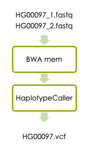
#It is recommended to specify the tool version for reproducibility, although not required1 Part1: Variant calling in one sample
Now let’s start the first part of the exercise, which is variant calling in one sample. The workflow consists of aligning the reads with BWA and detecting variants with HaplotypeCaller as illustrated below.
1.1 Aligning to genome
Index the genome
Many tools need an index of the reference genome to work efficiently. You therefore need to create index files for each tool first.
Generate a BWA index, fasta index and a sequence dictionary:
bwa index -a bwtsw human_g1k_v37_chr2.fasta

samtools faidx human_g1k_v37_chr2.fasta

gatk --java-options -Xmx4g CreateSequenceDictionary -R human_g1k_v37_chr2.fasta -O human_g1k_v37_chr2.dict
Check what files were created using ls -lrt.
Mapping reads
You will use BWA mem to align the reads to the reference genome. You need to provide the reference fasta file and two fastq files (for paired reads).
bwa mem human_g1k_v37_chr2.fasta HG00097_1.fq HG00097_2.fq > HG00097.samSort the aligned reads by chromosome position and convert the sam file to bam format.
samtools sort HG00097.sam > HG00097.bamNext, you need to index the generated bam file so that programs can access the sorted data without reading the whole file.
samtools index HG00097.bamPlease check what output files have been generated using ls -lrt. Is there a size difference between the sam and the bam file?
Check sam and bam files
You can look at the sam file using “less”. The bam file, on the other hand, is binary so we need to use samtools view.
less HG00097.sam

#View the first 5 lines of the bam file
samtools view HG00097.bam | head -n 5

#The header section of the bam file can be viewed separately with the -H flag:
samtools view -H HG00097.bam
Question 1A
- The
@SQtag of the bam header contains information about the reference sequence. What do you think SN:2 and LN:243199373 in this tag means?
- What is the leftmost mapping position of the first read in the bamfile?
For more information about the format, please have a look at the Sequence Alignment/Map Format Specification.
1.2 Variant Calling
1.2.1 HaplotypeCaller
We will detect short variants in the bam file using GATK’s HaplotypeCaller. First you need to add something called a read group, which contains information about the samples and sequencing. Read groups are required by HaplotypeCaller. We will use toy information here, but the RGSM tag should contain the sample name, and the RGID should be unique for each sample and sequencing run. To learn more about read groups please read this article.
gatk AddOrReplaceReadGroups -I HG00097.bam -O HG00097.rg.bam \
--RGID rg_HG00097 --RGSM HG00097 --RGPL illumina --RGLB libx --RGPU XXX

#Index the resulting bam file
samtools index HG00097.rg.bam
Now you can run the variant calling:
gatk --java-options -Xmx4g HaplotypeCaller \
-R human_g1k_v37_chr2.fasta -I HG00097.rg.bam -O HG00097.vcf
Check what new files were generated using ls -lrt.
1.2.2 Explore the vcf file
Now you have your first vcf file containing the variants on chr2:136545000-136617000. Please look at the vcf file with less and try to understand its structure.
Vcf files contain meta-information lines starting with ##, a header line starting with #CHROM, and then data lines each containing information about one variant position in the genome. The header line defines the columns of the data lines. The meta-information lines starting with ##INFO define how the data in the INFO column is encoded, and the meta-information lines starting with ##FORMAT define how the data in the FORMAT column is encoded.
To view the different parts of the header you can try these commands:
grep '#CHROM' HG00097.vcf
grep '##INFO' HG00097.vcf
grep '##FORMAT' HG00097.vcf
To see only the variants you can use
grep -v "#" HG00097.vcf | head -n 5Questions 1B
- What column of the VCF file contains genotype information for the sample HG00097?
- What does GT in the FORMAT column of the data lines mean?
- What does AD in the FORMAT column of the data lines mean?
- What genotype does the sample HG00097 have at position 2:136545844? (Use “grep” to find it)
- What are the allelic depths for the reference and alternative alleles in sample HG00097 at position 2:136545844?
For more detailed information about vcf files please have a look at The Variant Call Format specification.
1.3 IGV visualization
Integrated Genomics Viewer (IGV) provides an interactive visualization of the reads in a bam file as well as variants in a vcf file. Here we will show you how to use IGV on your laptop.
Install IGV or use ThinLinc
(Precourse preparations) If you have not used IGV on your laptop before, then go to the IGV download page, and follow the instructions to download it. It will prompt you to fill in some information and agree to license. Launch the viewer through web start.
If you have problems with IGV locally, you can connect to Dardel via ThinLinc, however the number of licences for ThinLinc on Dardel is limited, so during the workshop it might not work for everyone.
1.3.1 Copy files to local workspace
If you use IGV on your laptop, you need to copy some files from Dardel to your laptop. First, create a local workspace on your laptop, for example a folder called vc_local on your desktop. You need to have write permission in this folder. The folder you created will be referred to as local workspace in this lab.
1.3.1.1 Download the bam file
You need to download the bam file and the corresponding .bai file to your laptop. Navigate to your local workspace (do not log in to Dardel). Copy the .bam and .bam.bai files you just generated with this command (replace username with your username):
scp username@dardel.pdc.kth.se:/cfs/klemming/projects/supr/naiss2025-22-1240/username/vc/HG00097.bam* .If scp does not work
Some users have problems with the wildcard “*”, try to write “HG00097.bam*”
Check that the files are now present in your local workspace using ls -lrt.
1.3.2 Bam files in IGV
Open IGV. In the upper left dropdown menu choose Human hg19 (which is the same as GRCh37).
In the File menu, select Load from File, navigate to your workspace, and select HG00097.bam. This data should now appear as a track in the tracks window.
You need to zoom in to see the reads. You can either select a region by click and drag, or by typing a region or a gene name in the text box at the top. We only have data for the region chr2:136545000-136617000, which covers the LTC gene, so you can type this region or the gene name in the search box .
1.3.3 Vcf files in IGV
Download the file HG00097.vcf to your local workspace as described for the bam file above.
Load the file HG00097.vcf into IGV as you did with the HG00097.bam file. You will now see all the variants called in HG00097. You can view variants in the LCT gene by typing the gene name in the search box, and you can look specifically at the variant at position chr2:136545844 by typing that position in the search box.
Questions 1C
- What is the read length?
- Approximately how many reads cover an arbitrary position in the genomic region we are looking at?
- Which genes are located within the region chr2:136545000-136617000?
- Hover the mouse over (or click) the upper row of the vcf track. What is the reference and alternative alleles of the variant at position chr2:136545844?
- Hover the mouse over the lower row of the vcf track and look under “Genotype Information”. What genotype does HG00097 have at position chr2:136545844? Is this the same as you found by looking directly in the vcf file in question 10?
- Look at the bam track and count the number of reads that have “G” and “C”, respectively, at position chr2:136545844. How is this information captured under “Genotype Attributes”? (Again, hover the mouse over the lower row of the vcf track.)
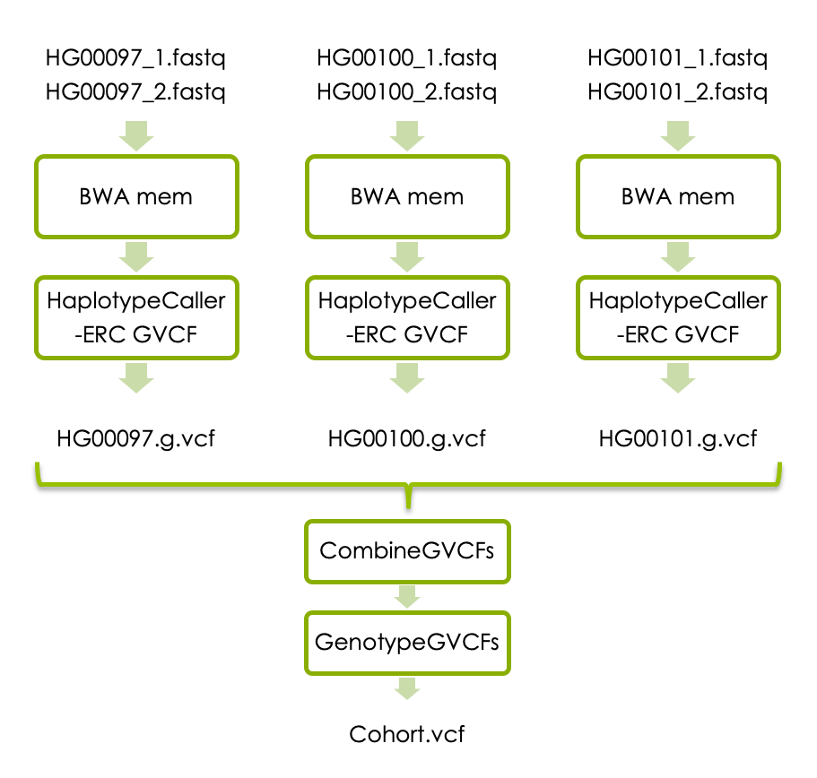
2 Part2: Variant calling in cohort
You will now try joint variant calling in three samples. Each sample will again be processed with BWA mem and HaplotypeCaller. We will however add a few steps and modify the variant calling to generate one g.vcf file per sample. The individual g.vcf files are combined with GATK’s CombineGVCFs, and translated into vcf format with GATK’s GenotypeGVCFs. The workflow below shows how the three samples are processed and combined.
2.1 Mapping - cohort
2.1.1 Alignment
We will run bwa a bit differently this time: mapping, sorting and conversion to bam will be performed in a single line. You will also add the read group information already in this step.
In addition, you can specify how many threads the program should use, which should be the same as the number of cores that you have access to. As we have asked for 8 cores we can specify -t 8 below.
Remember to replace sample with the sample name, both in the read group and in file names.
bwa mem -t 8 \
-R "@RG\tID:rg_sample\tSM:sample\tPU:XXX\tLB:libx\tPL:illumina" \
human_g1k_v37_chr2.fasta sample_1.fq sample_2.fq | samtools sort > sample.bam
Exact command for the first sample
bwa mem -t 8 -R "@RG\tID:rg_HG00097\tSM:HG00097\tPU:XXX\tLB:libx\tPL:illumina" human_g1k_v37_chr2.fasta HG00097_1.fq HG00097_2.fq | samtools sort > HG00097.bamPlease check what output files were generated this time. What could the advantage be of running it in one line?
2.1.2 Mark Duplicates
Sometimes the same DNA fragment is sequenced multiple times, which leads to multiple reads from the same fragment in the fastq files. If a duplicated read contains a genetic variant, the ratio of the two alleles might be obscured, which can lead to incorrect genotyping. It is therefore recommended (in most cases) to mark duplicate reads so that they are counted as one during genotyping. Please read about Picard’s MarkDuplicates here.
Run MarkDuplicates on all three bam files generated in the previous step.
gatk --java-options -Xmx4g MarkDuplicates \
    -I sample.bam -O sample.md.bam -M sample_mdmetrics.txt

samtools index sample.md.bam
2.2 Variant calling - cohort
2.2.1 Generate g.vcf files
HaplotypeCaller should also be run for all three samples, but this time the output for each sample needs to be in g.vcf format. This is accomplished by adding the -ERC GVCF flag.
gatk --java-options -Xmx4g HaplotypeCaller -R human_g1k_v37_chr2.fasta \
-ERC GVCF -I sample.md.bam -O sample.g.vcf
2.2.2 Joint genotyping
Once you have the g.vcf files for all samples you should perform joint genotype calling. To do this you first need to combine all individual .g.vcf files to one file using CombineGVCFs. Remember to replace sample1, sample2, sample3 with the real sample names.
gatk --java-options -Xmx4g CombineGVCFs -R human_g1k_v37_chr2.fasta \
-V sample1.g.vcf -V sample2.g.vcf -V sample3.g.vcf -O cohort.g.vcf
Then run GenoteypeGVC to generate a vcf file:
gatk --java-options -Xmx4g GenotypeGVCFs -R human_g1k_v37_chr2.fasta \
-V cohort.g.vcf -O cohort.vcf
Questions 2A
- How many data lines does the cohort.g.vcf file have? You can use the Linux command
grep -v "#" cohort.g.vcf | wc -lto extract and count lines in “cohort.g.vcf” that don’t start with “#”.
- How many data lines does the cohort.vcf file have? Explain the difference in number of lines.
- What is encoded in the last three columns of the data lines?
2.3 Variant filtration
HaplotypeCaller is designed to be very sensitive, which minimizes the risk of missing real variants. However, it means that the number of false positives can be quite large, so we need to filter the raw variant set. There are more sophisticated tools in the GATK suite for this, but we will use a simple filter, based on the quality value.
gatk --java-options -Xmx4g VariantFiltration -R human_g1k_v37_chr2.fasta \
  -V cohort.vcf -O cohort.filtered.vcf \
  --filter-name QUALfilt --filter-expression "QUAL < 100"
Note that the FILTER column is now filled.
vcftools is another tool that can be used to filter and manipulate the vcf file. For example, variants that did not pass the filters can be removed, and we can add other filters, for example mean sequencing depth.
vcftools --vcf cohort.filtered.vcf --remove-filtered-all --min-meanDP 5 --recode --recode-INFO-all --out cohort.PASSSee the vcftools manual for more options.
Questions 2B
- Check how many variants in total that are present in the cohort.filtered.vcf file and how many that have passed the filters. Is the difference big?
- Look at the variants that did not pass the filters using
grep -v 'PASS' cohort.filtered.vcf. (Do you understand why these variants didn’t pass the filter?)
- How many variants were removed by vcftools (in cohort.PASS.recode.vcf)?
- Try to remove all indels using vcftools. How many variants remain?
2.4 IGV visualization of cohort vcf
Again, you have to download the files to your local workspace to look at them in IGV. This time you will view cohort.filtered.vcf, HG00097.md.bam, HG00100.md.bam and HG00101.md.bam and the corresponding index files.
Load the files into IGV as described earlier. This time let us look closer at the lactase persistence related variant, rs4988235, located at position chr2:136608646. Please use IGV to answer the questions below.
Questions 2C
- What is the reference and alternative alleles at chr2:136608646?
- What genotypes do the three samples have at chr2:136608646? Note how genotypes are color coded in IGV.
- Should any of the individuals avoid drinking milk (i.e. homozygous reference)?
- Now compare the data shown in IGV with the data in the VCF file. Extract the row for the chr2:136608646 variant in the cohort.vcf file, for example using
grep '136608646' cohort.vcf. What columns of the vcf file contain the information shown in the upper part of the vcf track in IGV?
- What columns of the vcf file contain the information shown in the lower part of the vcf track?
- Zoom out so that you can see the MCM6 and LCT genes. Is the variant at chr2:136608646 located within the LCT gene?
When you have finished the exercises, you can have a look at this document with answers to all questions, and compare them with your answers.
3 Part3: SBATCH scripts
This section is optional and intended for those who want to learn how to run all steps automatically in a bash script. Please make sure that you have understood all the individual steps before you start with this. To learn more about SLURM and SBATCH scripts please look at the How to Run Jobs page on the PDC website.
Variant calling in cohort
Below is a skeleton script that can be used as a template for running variant calling in a cohort. Modify it to run all the steps in part two of this workshop.
#!/bin/bash
#SBATCH -A naiss2025-22-1240
#SBATCH -p shared
#SBATCH -c 8
#SBATCH -t 1:00:00
#SBATCH -J JointVariantCalling

module load bioinfo-tools
module load bwa/0.7.17
module load samtools/1.20
module load gatk/4.5.0.0

## loop through the samples:
for sample in HG00097 HG00100 HG00101;
do
  echo "Now analyzing: "${sample}
  #Fill in the code for running bwa-mem for each sample here
  #Fill in the code for samtools index for each sample here
  #Fill in the code for MarkDuplicates here
  #Fill in the code for HaplotypeCaller for each sample here
done
#Fill in the code for CombineGVCFs for all samples here
#Fill in the code for GenotypeGVCFs here
Save the template in your workspace and call it “joint_genotyping.sbatch” . Make the script executable by this command:
chmod u+x joint_genotyping.sbatchTo run the sbatch script in the SLURM queue, use this command:
sbatch joint_genotyping.sbatchIn this lab you have an active node reservation so you can also run the script as a normal bash script:
./joint_genotyping.sbatchIf you would like more help with creating the sbatch script, please look at our example solution below (click on the link):
Example solution
#!/bin/bash
#SBATCH -A naiss2025-22-1240
#SBATCH -p shared
#SBATCH -c 8
#SBATCH -t 2:00:00
#SBATCH -J JointVariantCalling

module load bioinfo-tools
module load bwa/0.7.17
module load samtools/1.20
module load gatk/4.5.0.0

for sample in HG00097 HG00100 HG00101;
do
  echo "Now analyzing: "${sample}
  bwa mem -R \
  "@RG\tID:${sample}\tPU:flowcellx_lanex\tSM:${sample}\tLB:libraryx\tPL:illumina" \
  -t 8 human_g1k_v37_chr2.fasta "${sample}_1.fq" "${sample}_2.fq" | samtools sort > "${sample}.bam"

  samtools index "${sample}.bam"

  gatk --java-options -Xmx4g MarkDuplicates \
  -R human_g1k_v37_chr2.fasta \
  -I "${sample}.bam" \
  -O "${sample}.md.bam" \
  -M "${sample}_mdmetrics.txt"


  gatk --java-options -Xmx4g HaplotypeCaller \
  -R human_g1k_v37_chr2.fasta \
  -ERC GVCF -I "${sample}.bam" \
  -O "${sample}.g.vcf"

done

gatk --java-options -Xmx4g CombineGVCFs \
-R human_g1k_v37_chr2.fasta \
-V HG00097.g.vcf \
-V HG00100.g.vcf \
-V HG00101.g.vcf \
-O cohort.g.vcf

gatk --java-options -Xmx4g GenotypeGVCFs \
-R human_g1k_v37_chr2.fasta \
-V cohort.g.vcf \
-O cohort.vcf
4 Extra material: GATK’s best practices
If you receive your sequencing data with variants called, it is likely that your data has been processed according to the GATKs best practices for germline short variant discovery. GATK is often used for human sequencing data, but also for many other organisms, especially model organisms. If you are interested you can try this optional section, where the variant calling is refined further.
GATK best practises germline variant calling
This will be included in the lecture on Thursday morning. If you reach this step earlier you can have a look at this prerecorded video of the same lecture.
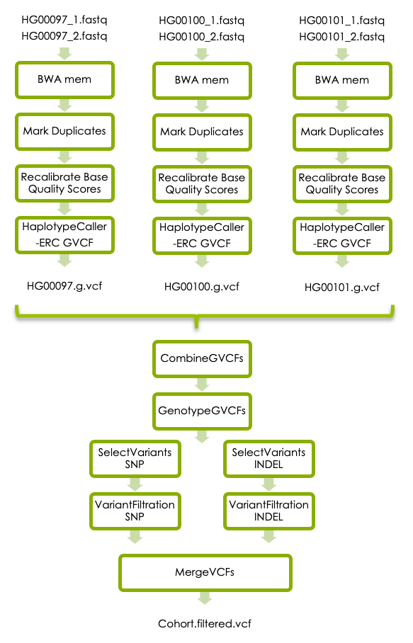
4.1 Mapping - GATK Best practise
BWA mem
The first step in GATK’s best practice variant calling workflow is to run BWA mem and MarkDuplicates for each sample exactly as you did in Variant calling in cohort. You have already done this step, so please use the bam files that you generated before (sample.md.bam).
Recalibrate Base Quality Scores
A potential source of error is systematic biases in the assignment of base quality scores by the sequencing instrument. This can be corrected by GATK’s Base Quality Score Recalibration. In short, you first use BaseRecalibrator to build a recalibration model, and then ApplyBQSR to recalibrate the base qualities in your bam file.
BaseRecalibrator requires a file with known SNPs as input. This file is available in the data folder on Dardel. Make a soft link to this file:
ln -s /sw/courses/ngsintro/vc/data/ref/1000G_phase1.snps.high_confidence.b37.chr2.vcfFirst, run BaseRecalibrator for the bam file generated in the previous step:
gatk --java-options -Xmx4g BaseRecalibrator -R human_g1k_v37_chr2.fasta \
      --known-sites 1000G_phase1.snps.high_confidence.b37.chr2.vcf \
      -I HG00097.md.bam -O HG00097.recal.table
Then run ApplyBQSR:
gatk --java-options -Xmx4g ApplyBQSR -R human_g1k_v37_chr2.fasta \
    -bqsr-recal-file HG00097.recal.table \
    -I HG00097.md.bam -O HG00097.recal.bam
Repeat for all three samples
4.2 Variant calling - GATK Best Practise
Generate g.vcf files
Next, HaplotypeCaller should be run for all three samples, and the output should be in g.vcf, as described above. This time use the recalibrated bam files as input.
Joint genotyping
Once you have the g.vcf files for all samples you should perform joint genotype calling. This is done with CombineGVCFs and GenotypeGVCFs as described above, but you should use the g.vcf files generated from the recalibrated bam files as input.
Variant Filtration
GATK offers two ways to filter variants:
The variant quality score recalibration (VQSR) method uses machine learning to identify variants that are likely to be real. This is the best method if you have a lot of data, for example one whole genome sequence sample or several whole exome samples, and work with human, mouse or any other well-studied organism. Read more here GATK VQSR
If you have less data, or a non-model organism, you can use hard filters as described here.
Since we have very little data we will use hard filters. The parameters are slightly different for SNVs and INDELs, so you need to first select all SNVs using SelectVariants and filter them using VariantFiltration with the parameters suggested for SNVs, and then the same for indels. Finally merge the SNVs and INDELs to get all variants in one file. The cutoffs are suggested starting values, but should be adjusted to the dataset. Read about hard filters here.
4.2.1 Hard filters
Example solution for filtering SNVs:
gatk --java-options -Xmx4g SelectVariants \
  -R human_g1k_v37_chr2.fasta \
  --select-type-to-include SNP \
  -V cohort.vcf -O cohort.snvs.vcf

gatk --java-options -Xmx4g VariantFiltration \
  -R human_g1k_v37_chr2.fasta \
  -V cohort.snvs.vcf -O cohort.snvs.filtered.vcf \
  --filter-name QDfilter --filter-expression "QD < 2.0"  \
  --filter-name MQfilter --filter-expression "MQ < 40.0"  \
  --filter-name FSfilter --filter-expression "FS > 60.0"
Example filters for INDELs:
gatk --java-options -Xmx4g SelectVariants \
  -R human_g1k_v37_chr2.fasta \
  -V cohort.vcf -O cohort.indels.vcf \
--select-type-to-include INDEL \


gatk --java-options -Xmx4g VariantFiltration \
  -R human_g1k_v37_chr2.fasta \
  -V cohort.indels.vcf -O cohort.indels.filtered.vcf \
  --filter-name QDfilter --filter-expression "QD < 2.0" \
  --filter-name FSfilter --filter-expression "FS > 200.0"
Merge filtered SNPs and INDELs:
gatk --java-options -Xmx4g MergeVcfs \
    -I cohort.snvs.filtered.vcf -I cohort.indels.filtered.vcf -O cohort.filtered.vcf
Look at your filtered vcf with e.g. less. It still has all the variant lines, but the FILTER column is now filled in, with PASS or the filters it failed. Note also that the filters that were run are described in the header section.
5 When finished
Clean up
When the analysis is done and you are sure that you have the desired output, it is a good practice to remove intermediary files that are no longer needed. This will save disk space, and will be a crucial part of the routines when you work with your own data. Please think about which files you need to keep if you would like to go back and look at this lab later on. Remove the other files.
Answers
When you have finished the exercise, please have a look at this document with answers to all questions, and compare them with your answers.
Additional information
Precomputed files
If you run out of time you can click below to get paths to precomputed bam files.
Precomputed files
/sw/courses/ngsintro/vc/data/bam/HG00097.bam
/sw/courses/ngsintro/vc/data/bam/HG00100.bam
/sw/courses/ngsintro/vc/data/bam/HG00101.bam
If you run out of time you can click below to get paths to the precomputed cohort.g.vcf and cohort.vcf files.
/sw/courses/ngsintro/vc/data/vcf/cohort.g.vcf
/sw/courses/ngsintro/vc/data/vcf/cohort.vcf
If you run out of time, please click below to get the path to precomputed bam and vcf files for the GATK’s best practices section.
Path to intermediary and final bam files: /sw/courses/ngsintro/vc/data/best_practise_bam
Path to intermediary and final vcf files: /sw/courses/ngsintro/vc/data/best_practise_vcf- Here is a technical documentation of Illumina Quality Scores
- Tools used or referenced
Thanks for today!