Variant Calling Workflow
From reads to short variants
Introduction
Whole genome sequencing (WGS) is a comprehensive method for analyzing entire genomes. This workshop will take you through the process of calling germline short variants (SNVs and INDELs) in WGS data from three human samples.
- The first part of the workshop will guide you through a basic variant calling workflow in one sample. The goals are that you should get familiar with the bam and vcf file formats, and learn how to interpret the results of variant calling in Integrative Genomics Viewer (IGV).
- If you have time, the next part of the workshop will show you how to perform joint variant calling in three samples. The goals here is that you should be able to interpret multi-sample vcf files and explain the differences between the g.vcf and vcf file formats. Also, if you are interested in programming, another goal is that you should learn to combine individual Linux commands into an SBATCH script.
- If you have time, the last part of the workshop will take you through the GATK best practices for germline short variant detection in three samples. The goal here is that you should learn how to use GATK’s documentation so that you can analyze your own samples in the future.
- You will work on the computing cluster Rackham at Uppmax
- In paths, please replace
<username>with your actual UPPMAX username. - In commands, please replace
<parameter>with the correct parameter, for example your input file name, output file name, directory name, etc. - Do not copy and paste commands from the exercise to terminal, as this can result in formatting errors.
- Use tab completion.
- A line starting with
#is a comment - Running a command without parameters will often return a help message on how to run the command.
- After a command is completed, please check that the desired output file was generated and that it has a reasonable size (use
ls -l). - A common mistake is to attempt to load input files that do not exist, or create output files where you don’t have permission to write.
- Use output file names that describes what was done in the command.
- If you change the node you are working on you will need to reload the tool modules.
- Google errors, someone in the world has run into EXACTLY the same problem you had and asked about it on a forum somewhere.
Data description
Samples
The 1000 Genomes Project ran between 2008 and 2015, creating the largest public catalogue of human variation and genotype data. In this workshop we will use low coverage whole genome sequence data from three individuals, generated in the first phase of the 1000 Genomes Project.
| Sample | Population | Sequencing technology |
|---|---|---|
| HG00097 | British in England and Scotland | Low coverage WGS |
| HG00100 | British in England and Scotland | Low coverage WGS |
| HG00101 | British in England and Scotland | Low coverage WGS |
Genomic region
The LCT gene on chromosome 2 encodes the enzyme lactase, which is responsible for the metabolism of lactose in mammals. Most mammals can not digest lactose as adults, but some humans can. Genetic variants upstream of the LCT gene lead to lactase persistence, which means that lactase is expressed also in adulthood and the carrier can continue to digest lactose. The variant rs4988235, located at position chr2:136608646 in the HG19 reference genome, has been shown to lead to lactose persistence. The alternative allele (A on the forward strand and T on the reverse strand) creates a new transcription factor binding site that enables continued expression of the gene after weaning.
In this workshop we will use sequencing data for the region chr2:136545000-136617000 chr2:136,039,147-136,662,073 in the 3 samples listed above to illustrate variant calling in NGS data. We will use chromosome 2 from hg19 as reference genome.
For those interested in the details of the genetic bases for lactose tolerance, please read the first three pages of Lactose intolerance: diagnosis, genetic, and clinical factors by Mattar et al. The variant rs4988235 is here referred to as LCT-13910C>T.
Data folder on UPPMAX
All input data for this exercise is located in this folder on Rackham:
/sw/courses/ngsintro/reseq/dataThe fastq files are located in this folder:
/sw/courses/ngsintro/reseq/data/fastqReference files, such as the reference genome in fasta format, are located in this folder:
/sw/courses/ngsintro/reseq/data/refPreparations
Local workspace
The majority of the analyses in this workshop will be done on UPPMAX, but you will copy some of the resulting files to your laptop. Therefore, please start by creating a folder for this workshop on your laptop, for example a folder called ngsworkflow on Desktop. You need to have write permission in this folder. The folder you create here will be referred to as local workspace throughout this workshop.
For MobaXterm users
MobaXterm users need to set the persistent home directory to your local workspace. This means that your home directory in MobaXterm will be set to the folder that you created in the previous step.
- In MobaXterm click on the Settings tab, then choose Configurations.
- Click on the yellow folder icon in the line of Persistent home directory. Browse to the desired folder and click on OK.
- Then click OK to exit the Configurations window.
- Let MobaXterm restart to make the settings effective.
Now your MobaXterm home directory is set to the folder you created for this lab. More details about this can be found in this video
UPPMAX
Please connect to the Rackham cluster on UPPMAX using ssh:
$ ssh -Y username@rackham.uppmax.uu.seWorkspace on UPPMAX
Start by creating a workspace for this exercise in your folder under the course’s nobackup folder, and then move into it. This folder will be referred to as your UPPMAX workspace throughout this workshop.
mkdir /proj/g2021013/nobackup/<username>/ngsworkflow
cd /proj/g2021013/nobackup/<username>/ngsworkflow
Symbolic links to data
The raw data files are located in the Data folder described above.
Create a symbolic link to the reference genome in your workspace:
ln -s /sw/courses/ngsintro/reseq/data/ref/human_g1k_v37_chr2.fastaDo the same with the fastq files:
ln -s /sw/courses/ngsintro/reseq/data/fastq/HG00097_1.fq
ln -s /sw/courses/ngsintro/reseq/data/fastq/HG00097_2.fq
ln -s /sw/courses/ngsintro/reseq/data/fastq/HG00100_1.fq
ln -s /sw/courses/ngsintro/reseq/data/fastq/HG00100_2.fq
ln -s /sw/courses/ngsintro/reseq/data/fastq/HG00101_1.fq
ln -s /sw/courses/ngsintro/reseq/data/fastq/HG00101_2.fq
Book a node
Book a compute node (or actually just one core of a node) so that you can run compute intensive tasks in the terminal. Make sure you only do this once each day because we have reserved one core per student for the course.
Use this reservation on day 1 of variant-calling:
salloc -A g2021013 -t 04:00:00 -p core -n 1 --no-shell --reservation=g2021013_19 &Use this reservation on day 2 of variant-calling:
salloc -A g2021013 -t 04:00:00 -p core -n 1 --no-shell --reservation=g2021013_20 &Once your job allocation has been granted (should not take long) you can connect to the node using ssh. To find out the name of your node, use:
squeue -u <username>The node name is found under nodelist header, you should only see one. Connect to that node:
ssh -Y <nodename>Accessing programs
Load the modules that are needed during this workshop. Remember that these modules must be loaded every time you login to Rackham, or when you connect to a new compute node.
First load the bioinfo-tools module:
module load bioinfo-toolsThis makes it possible to load the individual programs:
module load FastQC/0.11.8
module load bwa/0.7.17
module load samtools/1.10
module load GATK/4.1.4.1
Although you don’t have to specify which versions of the tools to use, it is recommended to do so for reproducibility if you want to rerun the exact same analyses later.
When loading the module GATK/4.1.4.1 you will get a warning message about the fact that GATK commands have been updated since the previous version of GATK. This is fine and you don’t have to do anything about it.
Index the genome
Tools that compare short reads with a large reference genome needs indexes of the reference genome to work efficiently. You therefore need to create index files for each tool.
Generate BWA index files:
bwa index -a bwtsw human_g1k_v37_chr2.fastaCheck to see that several new files have been created using ls -l.
Generate a samtools index:
samtools faidx human_g1k_v37_chr2.fastaCheck to see what file(s) were created using ls -lrt.
Generate a GATK sequence dictionary:
gatk --java-options -Xmx7g CreateSequenceDictionary -R human_g1k_v37_chr2.fasta -O human_g1k_v37_chr2.dictAgain, check what file(s) were created using ls -lrt.
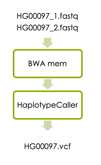
1 Variant calling in one sample
Now let’s start the main part of the workshop, which will guide you through a basic variant calling workflow in one sample. The workflow consists of aligning the reads with BWA and detecting variants with HaplotypeCaller as illustrated below.
1.1 Aligning reads
1.1.1 BWA mem
You should use BWA mem to align the reads to the reference genome.
In the call to BWA mem you need to add something called a read group, which contains information about how the reads were generated. This is required by HaplotypeCaller. Since we don’t know exactly how the reads in the 1000 Genomes Project were generated we have to make some assumptions. Let’s assume that each pair of fastq files was generated from one library preparation (libraryx), derived from one biological sample (HG00097), that was run on one lane of a flowcell on the Illumina machine (lanex_flowcellx) , and let’s define a read group with this information (readgroupx). The code for adding this read group is:
-R "@RG\\tID:readgroupx\\tPU:lanex_flowcellx\\tSM:HG00097\\tLB:libraryx\\tPL:illumina"When running BWA for another sample later on you have to replace HG00097 in the read group with the new sample name. To learn more about read groups please read this article at GATK forum.
You also need to specify how many threads the program should use (should be the same as the number of cores you have access to and is defined by the code -t 1 below), what reference genome file to use and what fasta files to align.
The output from BWA should be parsed to samtools sort, which sorts the sam file according to chromosome position and then converts the sam file to the binary bam format.
Finally, use a file redirect > so that the output ends up in a file and not on your screen.
Please use this command to align the reads, add the read group, sort the reads and write them to a bam file:
bwa mem -R "@RG\\tID:readgroupx\\tPU:lanex_flowcellx\\tSM:HG00097\\tLB:libraryx\\tPL:illumina" -t 1 human_g1k_v37_chr2.fasta HG00097_1.fq HG00097_2.fq | samtools sort > HG00097.bamPlease check that the expected output file was generated and that it has content using ls -lrt.
Next you need to index the output bam file so that programs can randomly access the sorted data without reading the whole file. This command creates an index file with the same name as the input bam file, except with a .bai extension:
samtools index HG00097.bamPlease check what output file was generated this time.
1.1.2 Check bam with samtools
The bam file is binary so we cannot read it, but we can view it with samtools view. The header section of the bam file can be viewed separately with the -H flag:
samtools view -H HG00097.bam To look at the reads in the bam file just use samtools view without the -H. This will display the entire bam file which is quite large, so if you just want to look at the first 5 lines (for example) you can combine samtools view with head:
samtools view HG00097.bam | head -n 5 For help with interpreting the bam file, please look at the sam/bam format definition at Sequence Alignment/Map Format Specification.
1.1.3 Questions
- What does “SO:coordinate” in the “@HD” tag on the first line of the bam file mean?
- What does “SN:2” and “LN:243199373” in the "@SQ tag mean?
- What is encoded in the @RG tag?
- What is the leftmost mapping position of the first read in the bamfile?
1.1.4 Check bam in IGV
Install IGV
Integrated Genomics Viewer (IGV) provides an interactive visualisation of the reads in a bam file. Here we will show you how to run IGV on your laptop. If you have not used IGV on your laptop before, then go to the IGV download page, and follow the instructions to download it. It will prompt you to fill in some information and agree to license. Launch the viewer through web start. The 1.2 Gb version should be sufficient for our data.
Download the bam file
You also need to download the bam file and the corresponding .bai file to your laptop. Navigate to your local workspace, but do not log in to UPPMAX. Copy the .bam and .bam.bai files you just generated with this command:
scp <username>@rackham.uppmax.uu.se:/proj/g2021013/nobackup/<username>/ngsworkflow/HG00097.bam* .Check that the files are now present in your local workspace using ls -lrt.
Look at the bam file in IGV
- In
IGV, go to the popup menu in the upper left and set it toHuman hg19.
- In the
Toolsmenu, selectRun igvtools. Choose the commandCountand then use theBrowsebutton next to theInput Fileline to select the bam file (not the bai) that you just downloaded. It will autofill the output file. Hit theRunbutton. This generates a .tdf file that allows you to see the coverage value for our bam file even at zoomed out views.Closethe igvtools window.
- In the
Filemenu, selectLoad from Fileand select your BAMs (not the .bai or the .tdf), which should appear in the tracks window. You will have to zoom in before you can see any reads. You can either select a region by click and drag, or by typing a region or a gene name in the text box at the top. Remember that we have data for the region chr2:136545000-136617000.
1.1.5 Questions
- What is the read length?
- How can you estimate the coverage at a specific position in IGV?
- Which RefSeq Genes are located within the region chr2:136545000-136617000?
1.2 Variant Calling
1.2.1 HaplotypeCaller
Now we will detect short variants in the bam file using GATK’s HaplotypeCaller. Go to your UPPMAX workspace and run:
gatk --java-options -Xmx7g HaplotypeCaller -R human_g1k_v37_chr2.fasta -I HG00097.bam -O HG00097.vcf Check what new files were generated with ls -lrt.
1.2.2 Explore the vcf file
Now you have your first vcf file containing the raw variants in the region chr2:136545000-136617000 in sample HG00097. Please look at the vcf file with less and try to understand its structure.
Vcf files contains meta-information lines starting with ##, a header line starting with #CHROM, and then data lines each containing information about one variant position in the genome. The header line defines the columns of the data lines, and to view the header line you can type this command:
grep '#CHROM' HG00097.vcfThe meta-information lines starting with ##INFO defines how the data in the INFO column is encoded, and the meta-information lines starting with ##FORMAT defines how the data in the FORMAT column is encoded. To view the meta-information lines describing the INFO column use:
grep '##INFO' HG00097.vcfTo view the meta-information lines describing the FORMAT column use:
grep '##FORMAT' HG00097.vcfNow lets look at the details of one specific genetic variant at position 2:136545844:
grep '136545844' HG00097.vcfFor more detailed information about vcf files please have a look at The Variant Call Format specification.
1.2.3 Questions
- What column of the VCF file contains genotype information for the sample HG00097?
- What does GT in the FORMAT column of the data lines mean?
- What genotype does the sample HG00097 have at position 2:136545844?
- What does AD in the FORMAT column of the data lines mean?
- What are the allelic depths for the reference and alternative alles in sample HG00097 at position 2:136545844?
- How many genetic variants was detected in the sample? The linux command
grep -v "#" HG00097.vcf | wc -lextracts all lines in HG00097.vcf that don’t start with “#”, and counts these lines.
1.2.4 Check vcf in IGV
Download the vcf file and its index to the local workspace on your laptop, just like you did with the bam file and its index earlier. Navigate to your local workspace, but do not log in to UPPMAX. Copy the files that you just generated:
scp <username>@rackham.uppmax.uu.se:/proj/g2021013/nobackup/<username>/ngsworkflow/HG00097.vcf* .Please replace <username> with your UPPMAX user name.
Note that the * in the end of the file name means that you will download all files that start with HG00097.vcf, so you will also download the vcf index.
Check that the files were properly downloaded to your local workspace using ls -lrt.
In IGV, in the File menu, select Load from File and select your vcf file (not the .idx file) and the bam file (not the .bai file) that you downloaded earlier. The vcf and bam files should appear in the tracks window. You will now see all the variants called in HG00097. You can view all variants in the LCT gene by typing the gene name in the search box, and you can look specifically at the variant at position chr2:136545844 by typing that position in the search box.
1.2.5 Questions
- Hoover the mouse over the upper row of the vcf track. What is the reference and alternative alleles of the variant at position chr2:136545844?
- Hoover the mouse over the lower row of the vcf track and look under “Genotype Information”. What genotype does HG00097 have at position chr2:136545844? Is this the same as you found by looking directly in the vcf file in question 10?
- Look in the bam track and count the number of reads that have “T” and “C”, respectively, at position chr2:136545844. How is this information captured under “Genotype Attributes”? (Again, hoover the mouse over the lower row of the vcf track.)
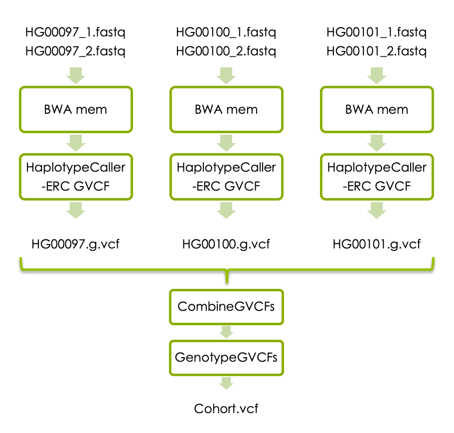
2 Variant calling in cohort
If you have time, you can now try joint variant calling in all three samples. Each sample has to be processed with BWA mem as above, and then with HaplotypeCaller with the flag -ERC to generate one g.vcf file per sample. The individual g.vcf files should subsequently be combined with GATK’s CombineGVCFs, and translated into vcf format with GATK’s GenotypeGVCFs. The workflow below shows how the three samples should be processed and combined.
You can run the commands one by one in the terminal as you did before. We have also made intermediary files available in case you don’t have time to complete all steps, please see links under each analysis step.
Optional: If you are interested in programming and have time, you can also try to write a simple SBATCH script and run all steps automatically. Please check out the SBATCH script section below if you would like to try this.
2.1 BWA mem
Run BWA mem for all three samples in the data set. BWA mem should be run exactly as above but with the new sample names. Please note that you also need to adjust the SM field in the read group so that it matches the new sample name, otherwise the joint genotyping step will not work properly.
If you run out of time, please click below to get paths to precomputed bam files.
/sw/courses/ngsintro/reseq/data/bam/HG00097.bam
/sw/courses/ngsintro/reseq/data/bam/HG00100.bam
/sw/courses/ngsintro/reseq/data/bam/HG00101.bam
2.2 Generate g.vcf files
HaplotypeCaller should also be run for all three samples, but this time the output for each sample needs to be in g.vcf format. This is accomplished with a small change in the HaploteypCaller command:
gatk --java-options -Xmx7g HaplotypeCaller -R human_g1k_v37_chr2.fasta -ERC GVCF -I <sample.bam> -O <sample>.g.vcf Please replace
If you run out of time, please click below to get paths to the precomputed g.vcf files.
/sw/courses/ngsintro/reseq/data/vcf/HG00097.g.vcf
/sw/courses/ngsintro/reseq/data/vcf/HG00100.g.vcf
/sw/courses/ngsintro/reseq/data/vcf/HG00101.g.vcf
2.3 Joint genotyping
Once you have the g.vcf files for all samples you should perform joint genotype calling. To do this you first need to combine all individual .g.vcf files to one file using CombineGVCFs:
gatk --java-options -Xmx7g CombineGVCFs -R human_g1k_v37_chr2.fasta -V <sample1>.g.vcf -V <sample2>.g.vcf -V <sample3>.g.vcf -O cohort.g.vcfPlease replace <sample1>, <sample2>, <sample3> with the real sample names.
Then run GATK’s GenoteypeGVC to generate a vcf file:
gatk --java-options -Xmx7g GenotypeGVCFs -R human_g1k_v37_chr2.fasta -V cohort.g.vcf -O cohort.vcfIf you run out of time, please click below to get paths to the precomputed cohort.g.vcf and cohort.vcf files.
/sw/courses/ngsintro/reseq/data/vcf/cohort.g.vcf
/sw/courses/ngsintro/reseq/data/vcf/cohort.vcf
2.3.1 Questions
- How many data lines do the cohort.g.vcf file have? You can use the Linux command
grep -v "#" cohort.g.vcfto extract all lines in “cohort.g.vcf” that don’t start with “#”, then|, and thenwc -lto count those lines.
- How many data lines do the cohort.vcf file have?
- Explain the difference in number of data lines.
- Look at the header line of the cohort.vcf file. What columns does it have?
- What is encoded in the last three columns of the data lines?
2.4 SBATCH script
Optional
This section is only for those of you who want to try to run all steps automatically in bash scripts.
To learn more about SLURM and SBATCH scripts please look the SLURM user guide on UPPMAX website.
Below is a skeleton script that can be used as a template. Please modify it to run all the steps in part two of this workshop.
#!/bin/bash
#SBATCH -A g2019031
#SBATCH -p core
#SBATCH -n 1
#SBATCH -t 1:00:00
#SBATCH -J jointGenotyping
module load bioinfo-tools
module load bwa/0.7.17
module load samtools/1.10
module load GATK/4.1.4.1
## loop through the samples:
for sample in HG00097 HG00100 HG00101;
do
  echo "Now analyzing: "$sample
  #Fill in the code for running bwa-mem for each sample here
  #Fill in the code for samtools index for each sample here
  #Fill in the code for HaplotypeCaller for each sample here
done
#Fill in the code for CombineGVCFs for all samples here
#Fill in the code for GenotypeGVCFs here
Please save the sbatch script in your UPPMAX folder and call it “joint_genotyping.sbatch” or similar. Make the script executable by this command:
chmod u+x joint_genotyping.sbatchTo run the sbatch script in the SLURM queue, use this command:
sbatch joint_genotyping.sbatchIf you have an active node reservation you can run the script as a normal bash script:
./joint_genotyping.sbatchIf you would like more help with creating the sbatch script, please look at our example solution:
#!/bin/bash
#SBATCH -A g2019031
#SBATCH -p core
#SBATCH -n 1
#SBATCH -t 1:00:00
#SBATCH -J jointGenotyping

module load bioinfo-tools
module load bwa/0.7.17
module load samtools/1.10
module load GATK/4.1.4.1

for sample in HG00097 HG00100 HG00101;
do
  echo "Now analyzing: "$sample
  bwa mem -R "@RG\tID:readgroupx\tPU:flowcellx_lanex\tSM:"$sample"\tLB:libraryx\tPL:illumina" -t 1 human_g1k_v37_chr2.fasta $sample"_1.fq" $sample"_2.fq" | samtools sort > $sample".bam"
  samtools index $sample".bam"
  gatk --java-options -Xmx7g HaplotypeCaller -R human_g1k_v37_chr2.fasta -ERC GVCF -I $sample".bam" -O $sample".g.vcf"
done
gatk --java-options -Xmx7g CombineGVCFs -R human_g1k_v37_chr2.fasta -V HG00097.g.vcf -V HG00100.g.vcf -V HG00101.g.vcf -O cohort.g.vcf
gatk --java-options -Xmx7g GenotypeGVCFs -R human_g1k_v37_chr2.fasta -V cohort.g.vcf -O cohort.vcf
Please answer the questions above.
2.5 Check combined vcf file in IGV
Download the file cohort.vcf and its index, as well as HG00100.bam and HG00101.bam and their indexes to your local workspace as described above. Then open cohort.vcf, HG00097.bam, HG00100.bam and HG00101.bam in IGV as described above. This time lets look at the variant rs4988235, located at position chr2:136608646 in the HG19 reference genome, that has been shown to lead to lactose persistence.
2.5.1 Questions
- What is the reference and alternative alleles at chr2:136608646?
- What genotype do the three samples have at chr2:136608646? Note how genotypes are color coded in IGV.
- Should any of the individuals avoid drinking milk?
- Now compare the data shown in IGV with the data in the VCF file. Extract the row for the chr2:136608646 variant in the cohort.vcf file, for example using
grep '136608646' cohort.vcf. What columns of the vcf file contain the information shown in the upper part of the vcf track in IGV? - What columns of the vcf file contain the information shown in the lower part of the vcf track?
- Zoom out so that you can see the MCM6 and LCT genes. Is the variant at chr2:136608646 locate within the LCT gene?
If you are interested in how this variant affects lactose tolerance please read the article by Mattar et al presented above, or in OMIM.
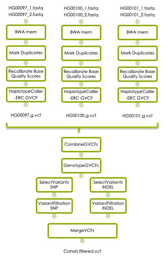
3 GATK’s best practices
The third part of this workshop will take you through additional refinement steps that are recommended in GATKs best practices for germline short variant discovery, illustrated in the flowchart below. You can either run the steps command by command in the terminal, or write an SBATCH script as described above.
The additional steps in the best practice workflow was not covered in the variant-calling lecture on Wednesday afternoon. There will be a short lecture about this on Thursday morning at 9 am. However, if you reach this step earlier you can have a look at this prerecorded video of the same lecture.
3.1 BWA mem
Run BWA mem for all three samples in the data set. BWA mem should be run exactly as above but with the new sample names. Please note that you also need to adjust the SM field in the read group so that it matches the new sample name.
3.2 Mark Duplicates
Sometimes the same DNA fragment is sequenced multiple times, which leads to multiple reads from the same fragment in the fastq file. This can occur due to PCR amplification in the library preparation, or if one read cluster is incorrectly detected as multiple clusters by the sequencing instrument. If a duplicated read contains a genetic variant, the ratio of the two alleles might be obscured, which can lead to incorrect genotyping. It is therefore recommended (in most cases) to mark duplicate reads so that they are counted as one during genotyping.
Please read about Picard’s MarkDuplicates here. Picard’s MarkDuplicates has recently been incorporated into the GATK suite, but the usage example in GATKs documentation still describes how to call it via the stand alone Picard program. A usage example for the version of MarkDuplicates that is incorporated in GATK is (with this you don’t have to load the Picard module):
gatk --java-options -Xmx7g MarkDuplicates \
      -I input.bam \
      -O marked_duplicates.bam \
      -M marked_dup_metrics.txt
If you would like more help you can sneak peek at our example solution for HG00097 below.
gatk --java-options -Xmx7g MarkDuplicates -I HG00097.bam -O HG00097.md.bam -M HG00097_mdmetrics.txt3.3 Recalibrate Base Quality Scores
Another source of error is systematic biases in the assignment of base quality scores by the sequencing instrument. This can be corrected by GATK’s Base Quality Score Recalibration.
In short, you first use BaseRecalibrator to build a recalibration model, and then ApplyBQSR to recalibrate the base qualities in your bam file.
BaseRecalibrator requires a file with known SNPs as input. This file is available in the data folder on UPPMAX:
/sw/courses/ngsintro/reseq/data/ref/1000G_phase1.snps.high_confidence.b37.chr2.vcfPlease use GATK’s documentation to recalibrate the base quality scores in your data. If you would like more help you can sneak peek at our example solution for HG00097 below.
gatk --java-options -Xmx7g BaseRecalibrator -R human_g1k_v37_chr2.fasta -I HG00097.md.bam --known-sites /sw/courses/ngsintro/reseq/data/ref/1000G_phase1.snps.high_confidence.b37.chr2.vcf -O HG00097.recal.table
gatk --java-options -Xmx7g ApplyBQSR -R human_g1k_v37_chr2.fasta -I HG00097.md.bam --bqsr-recal-file HG00097.recal.table -O HG00097.recal.bam
3.4 Generate g.vcf files
HaplotypeCaller should also be run for all three samples, and the output should be in g.vcf exactly as described above. This time use recalibrated bam files as input.
3.5 Joint genotyping
Once you have the g.vcf files for all samples you should perform joint genotype calling. This should be done with the commands CombineGVCFs and GenotypeGVCFs exactly as described above, but you should use the g.vcf files generated from the recalibrated bam files as input.
3.6 Variant Filtering
HaplotypeCaller is designed to be very sensitive, which is good because it minimizes the chance of missing real variants. However, it means that the number of false positives can be quite large, so we need to filter the raw callset. GATK offers two ways to filter variants:
1. The variant quality score recalibration (VQSR) method uses machine learning to identify variants that are likely to be real. This is the best method if you have a lot of data, for example one whole genome sequence sample or several whole exome samples.
2. If you have less data you can use hard filters as described here.
Since we have very little data we will use hard filters. The parameters are slightly different for SNVs and INDELs, so you need to first select all SNVs using SelectVariants and filter them using VariantFiltration with the parameters suggested for SNVs. Then select all INDELs and filter them with the parameters suggested for INDELs. Finally merge the SNVs and INDELs to get all variants in one file using MergeVCFs. If you would like more help you can sneak peek at our example solution for HG00097 below.
Filter SNVs:
gatk --java-options -Xmx7g SelectVariants
  -R human_g1k_v37_chr2.fasta
  -V cohort.vcf
  --select-type-to-include SNP
  -O cohort.snvs.vcf

gatk --java-options -Xmx7g VariantFiltration
  -R human_g1k_v37_chr2.fasta
  -V cohort.snvs.vcf
  -O cohort.snvs.filtered.vcf
  --filter-name QDfilter --filter-expression "QD < 2.0"
  --filter-name MQfilter --filter-expression "MQ < 40.0"
  --filter-name FSfilter --filter-expression "FS > 60.0"
Filter INDELs:
gatk --java-options -Xmx7g SelectVariants
  -R human_g1k_v37_chr2.fasta
  -V cohort.vcf
  --select-type-to-include INDEL
  -o cohort.indels.vcf

gatk --java-options -Xmx7g VariantFiltration
  -R human_g1k_v37_chr2.fasta
  -V cohort.indels.vcf
  -O cohort.indels.filtered.vcf
  --filter-name QDfilter --filter-expression "QD < 2.0"
  --filter-name FSfilter --filter-expression "FS > 200.0"
Merge filtered SNVs and INDELs:
gatk --java-options -Xmx7g MergeVcfs -I cohort.snvs.filtered.vcf -I cohort.indels.filtered.vcf -O cohort.filtered.vcfOpen your filtered vcf with less and page through it. It still has all the variant lines, but the FILTER column that was blank before is now filled in, with PASS or a list of the filters it failed. Note also that the filters that were run are described in the header section.
3.7 Precomputed files
If you run out of time, please click below to get the path to precomputed bam and vcf files for the GATK’s best practices section.
Path to intermediary and final bam files: /sw/courses/ngsintro/reseq/data/best_practise_bam
Path to intermediary and final vcf files: /sw/courses/ngsintro/reseq/data/best_practise_vcf
3.8 SBATCH script
We recommend you to incorporate the new steps into an SBATCH script similar to the one you created above for joint variant calling. Please try to complete the script for GATK’s best practices workflow. If you run out of time you can sneak peek at our example solution below.
#!/bin/bash
#SBATCH -A g2021013
#SBATCH -p core
#SBATCH -n 1
#SBATCH -t 1:00:00
#SBATCH -J BestPractise

## load modules
module load bioinfo-tools
module load bwa/0.7.17
module load samtools/1.10
module load GATK/4.1.4.1

# define path to reference genome
ref="/sw/courses/ngsintro/reseq/data/ref"

# make symbolic links
ln -s /sw/courses/ngsintro/reseq/data/ref/human_g1k_v37_chr2.fasta
ln -s /sw/courses/ngsintro/reseq/data/fastq/HG00097_1.fq
ln -s /sw/courses/ngsintro/reseq/data/fastq/HG00097_2.fq
ln -s /sw/courses/ngsintro/reseq/data/fastq/HG00100_1.fq
ln -s /sw/courses/ngsintro/reseq/data/fastq/HG00100_2.fq
ln -s /sw/courses/ngsintro/reseq/data/fastq/HG00101_1.fq
ln -s /sw/courses/ngsintro/reseq/data/fastq/HG00101_2.fq

# index reference genome
bwa index -a bwtsw human_g1k_v37_chr2.fasta
samtools faidx human_g1k_v37_chr2.fasta
gatk --java-options -Xmx7g CreateSequenceDictionary -R human_g1k_v37_chr2.fasta -O human_g1k_v37_chr2.dict

## loop through the samples:
for sample in HG00097 HG00100 HG00101;
do
  echo "Now analyzing: ${sample}"
  # map the reads
  bwa mem -R "@RG\tID:readgroupx\tPU:flowcellx_lanex\tSM:"$sample"\tLB:libraryx\tPL:illumina" -t 1 human_g1k_v37_chr2.fasta $sample"_1.fq" $sample"_2.fq" | samtools sort > $sample".bam"
  samtools index $sample".bam"
  # mark duplicates
  gatk --java-options -Xmx7g MarkDuplicates -I $sample".bam" -O $sample".md.bam" -M $sample"_mdmetrics.txt"
  # base quality score recalibration
  gatk --java-options -Xmx7g BaseRecalibrator -R human_g1k_v37_chr2.fasta -I $sample".md.bam" --known-sites $ref"/1000G_phase1.snps.high_confidence.b37.chr2.vcf" -O $sample".recal.table"
  gatk --java-options -Xmx7g ApplyBQSR -R human_g1k_v37_chr2.fasta -I $sample".md.bam" --bqsr-recal-file $sample".recal.table" -O $sample".recal.bam"
  # haplotypeCaller in -ERC mode
  gatk --java-options -Xmx7g HaplotypeCaller -R human_g1k_v37_chr2.fasta -ERC GVCF -I $sample".bam" -O $sample".g.vcf"
done

# joint genotyping
gatk --java-options -Xmx7g CombineGVCFs -R human_g1k_v37_chr2.fasta -V HG00097.g.vcf -V HG00100.g.vcf -V HG00101.g.vcf -O cohort.g.vcf
gatk --java-options -Xmx7g GenotypeGVCFs -R human_g1k_v37_chr2.fasta -V cohort.g.vcf -O cohort.vcf
# variant filtration SNPs
gatk --java-options -Xmx7g SelectVariants -R human_g1k_v37_chr2.fasta -V cohort.vcf --select-type-to-include SNP -O cohort.snvs.vcf
gatk --java-options -Xmx7g VariantFiltration -R human_g1k_v37_chr2.fasta -V cohort.snvs.vcf -O cohort.snvs.filtered.vcf --filter-name QDfilter --filter-expression "QD < 2.0" --filter-name MQfilter --filter-expression "MQ < 40.0"  --filter-name FSfilter --filter-expression "FS > 60.0"
# variant filtration indels
gatk --java-options -Xmx7g SelectVariants -R human_g1k_v37_chr2.fasta -V cohort.vcf --select-type-to-include INDEL -O cohort.indels.vcf
gatk --java-options -Xmx7g VariantFiltration -R human_g1k_v37_chr2.fasta -V cohort.indels.vcf -O cohort.indels.filtered.vcf --filter-name QDfilter --filter-expression "QD < 2.0" --filter-name FSfilter --filter-expression "FS > 200.0"
# merge filtered SNPs and indels
gatk --java-options -Xmx7g MergeVcfs -I cohort.snvs.filtered.vcf -I cohort.indels.filtered.vcf -O cohort.filtered.vcf
3.9 Questions
- How many variants are present in the cohort.filtered.vcf file?
- How many variants have passed the filters?
- Look at the variants that did not pass the filters using
grep -v 'PASS' cohort.filtered.vcf. Try to understand why these variants didn’t pass the filter.
Clean up
When the analysis is done and you are sure that you have the desired output, it is a good practice to remove intermediary files that are no longer needed. This will save disk space, and will be a crucial part of the routines when you work with your own data. Please think about which files you need to keep if you would like to go back and look at this lab later on. Remove the other files.
Answers
When you have finished the exercise, please have a look at this document with answers to all questions, and compare them with your answers.