3 Main exercise
The main exercise covers Differential Gene Expression (DGE) workflow from raw reads to a list of differentially expressed genes.
3.1 Using Uppmax
Connect to UPPMAX.
ssh -Y username@rackham.uppmax.uu.seBook a node.
For the RNA-Seq part of the course, we will work on the Rackham cluster. A standard compute node on cluster Rackham has 128 GB of RAM and 20 cores. We will use 1 core per person for this session. Therefore, each core gives you 6.4 GB of RAM. The code below is valid to run at the start of the day. If you are running it in the middle of a day, you need to decrease the time (-t). Do not run this twice and also make sure you are not running computations on a login node.
Book resources for RNA-Seq day 1.
salloc -A g2021013 -t 03:00:00 -p core -n 1 --reservation=g2021013_20Book resources for RNA-Seq day 2.
salloc -A g2021013 -t 04:00:00 -p core -n 1 --reservation=g2021013_213.1.1 Set-up directory
Setting up the directory structure is an important step as it helps to keep our raw data, intermediate data and results in an organised manner. All work must be carried out at this location /proj/g2021013/nobackup/<username>/ where <username> is your user name.
Create a directory named rnaseq. All RNA-Seq related activities must be carried out in this sub-directory named rnaseq.
mkdir rnaseqSet up the below directory structure in your project directory.
<username>/
rnaseq/
  +-- 1_raw/
  +-- 2_fastqc/
  +-- 3_mapping/
  +-- 4_qualimap/
  +-- 5_dge/
  +-- 6_multiqc/
  +-- reference/
  |   +-- mouse_chr19_hisat2/
  +-- scripts/
  +-- funannot/
  +-- plots
cd rnaseq
mkdir 1_raw 2_fastqc 3_mapping 4_qualimap 5_dge 6_multiqc reference scripts funannot plots
cd reference
mkdir mouse_chr19_hisat2
cd ..
The 1_raw directory will hold the raw fastq files (soft-links). 2_fastqc will hold FastQC outputs. 3_mapping will hold the mapping output files. 4_qualimap will hold the QualiMap output files. 5_dge will hold the counts from featureCounts and all differential gene expression related files. 6_multiqc will hold MultiQC outputs. reference directory will hold the reference genome, annotations and aligner indices. The funannot and plots directory are optional for bonus steps.
It might be a good idea to open an additional terminal window. One to navigate through directories and another for scripting in the scripts directory.
3.1.2 Create symbolic links
We have the raw fastq files in this remote directory: /sw/courses/ngsintro/rnaseq/main/1_raw/. We are going to create symbolic links (soft-links) for these files from our 1_raw directory to the remote directory. We do this because fastq files tend to be large files and simply copying them would use up a lot of storage space. Soft-linking files and folders allows us to work with those files as if they were actually there. Use pwd to check if you are standing in the correct directory. You should be standing here:
/proj/g2021013/nobackup/<username>/rnaseq/1_rawRun below to create softlinks. Note that the command ends in a space followed by a period.
ln -s /sw/courses/ngsintro/rnaseq/main/1_raw/*.gz .Check if your files have linked correctly. You should be able to see as below.
ls -lSRR3222409-19_1.fq.gz -> /sw/courses/ngsintro/rnaseq/main/1_raw/SRR3222409-19_1.fq.gz
SRR3222409-19_2.fq.gz -> /sw/courses/ngsintro/rnaseq/main/1_raw/SRR3222409-19_2.fq.gz
SRR3222410-19_1.fq.gz -> /sw/courses/ngsintro/rnaseq/main/1_raw/SRR3222410-19_1.fq.gz
SRR3222410-19_2.fq.gz -> /sw/courses/ngsintro/rnaseq/main/1_raw/SRR3222410-19_2.fq.gz
SRR3222411-19_1.fq.gz -> /sw/courses/ngsintro/rnaseq/main/1_raw/SRR3222411-19_1.fq.gz
SRR3222411-19_2.fq.gz -> /sw/courses/ngsintro/rnaseq/main/1_raw/SRR3222411-19_2.fq.gz
SRR3222412-19_1.fq.gz -> /sw/courses/ngsintro/rnaseq/main/1_raw/SRR3222412-19_1.fq.gz
SRR3222412-19_2.fq.gz -> /sw/courses/ngsintro/rnaseq/main/1_raw/SRR3222412-19_2.fq.gz
SRR3222413-19_1.fq.gz -> /sw/courses/ngsintro/rnaseq/main/1_raw/SRR3222413-19_1.fq.gz
SRR3222413-19_2.fq.gz -> /sw/courses/ngsintro/rnaseq/main/1_raw/SRR3222413-19_2.fq.gz
SRR3222414-19_1.fq.gz -> /sw/courses/ngsintro/rnaseq/main/1_raw/SRR3222414-19_1.fq.gz
SRR3222414-19_2.fq.gz -> /sw/courses/ngsintro/rnaseq/main/1_raw/SRR3222414-19_2.fq.gz3.2 FastQC
Quality check using FastQC
After receiving raw reads from a high throughput sequencing centre it is essential to check their quality. FastQC provides a simple way to do some quality control check on raw sequence data. It provides a modular set of analyses which you can use to get a quick impression of whether your data has any problems of which you should be aware before doing any further analysis.
Change into the 2_fastqc directory. Use pwd to check if you are standing in the correct directory. You should be standing here:
/proj/g2021013/nobackup/<username>/rnaseq/2_fastqcLoad Uppmax modules bioinfo-tools and FastQC FastQC/0.11.5.
module load bioinfo-tools
module load FastQC/0.11.8
Once the module is loaded, FastQC program is available through the command fastqc. Use fastqc --help to see the various parameters available to the program. We will use -o to specify the output directory path and finally, the name of the input fastq file to analyse. The syntax will look like below.
fastqc -o . ../1_raw/filename.fq.gzBased on the above command, we will write a bash loop to process all fastq files in the directory. Writing multi-line commands through the terminal can be a pain. Therefore, we will run larger scripts from a bash script file. Move to your scripts directory and create a new file named fastqc.sh.
You should be standing here to run this:
/proj/g2021013/nobackup/<username>/rnaseq/scriptsThe command below creates a new file in the current directory.
touch fastqc.shUse a text editor (nano,Emacs,gedit etc.) to edit fastqc.sh.
gedit behaves like a regular text editor with a standard graphical interface.
gedit fastqc.sh& Adding & at the end sends that process to the background, so that the console is free to accept new commands.
Then add the lines below and save the file.
#!/bin/bash

module load bioinfo-tools
module load FastQC/0.11.8

for i in ../1_raw/*.gz
do
    echo "Running $i ..."
    fastqc -o . "$i"
done
This script loops through all files ending in .gz. In each iteration of the loop, it executes fastqc on the file. The -o . flag to fastqc indicates that the output must be exported in this current directory.
While standing in the 2_fastqc directory, run the file fastqc.sh. Use pwd to check if you are standing in the correct directory.
You should be standing here to run this:
/proj/g2021013/nobackup/<username>/rnaseq/2_fastqcbash ../scripts/fastqc.shAfter the fastqc run, there should be a .zip file and a .html file for every fastq file. The .html file is the report that you need. Open the .html in the browser and view it. You do not need to necessarily look at all files now. We will do a comparison with all samples when using the MultiQC tool.
firefox file.html &Optional
Download the .html file to your computer and view it.
All users can use an SFTP browser like Filezilla or Cyberduck for a GUI interface. Windows users can also use the MobaXterm SFTP file browser to drag and drop.
Linux and Mac users can use SFTP or SCP by running the below command in a LOCAL terminal and NOT on Uppmax. Open a terminal locally on your computer, move to a suitable download directory and run the command below.
scp user@rackham.uppmax.uu.se:/proj/g2021013/nobackup/<username>/rnaseq/2_fastqc/SRR3222409_1_fastqc.html ./Go back to the FastQC website and compare your report with the sample report for Good Illumina data and Bad Illumina data.
Discuss based on your reports, whether your data is of good enough quality and/or what steps are needed to fix it.
3.3 HISAT2
Mapping reads using HISAT2
After verifying that the quality of the raw sequencing reads is acceptable, we will map the reads to the reference genome. There are many mappers/aligners available, so it may be good to choose one that is adequate for your type of data. Here, we will use a software called HISAT2 (Hierarchical Indexing for Spliced Alignment of Transcripts) as it is a good general purpose splice-aware aligner. It is fast and does not require a lot of RAM. Before we begin mapping, we need to obtain genome reference sequence (.fasta file) and build an aligner index. Due to time constraints, we will build an index only on chromosome 19.
3.3.1 Get reference
It is best if the reference genome (.fasta) and annotation (.gtf) files come from the same source to avoid potential naming conventions problems. It is also good to check in the manual of the aligner you use for hints on what type of files are needed to do the mapping. We will not be using the annotation (.gtf) during mapping, but we will use it during quantification.
What is the idea behind building an aligner index? What files are needed to build one? Where do we take them from? Could one use an index that was generated for another project? Check out the HISAT2 manual indexer section for answers. Browse through Ensembl and try to find the files needed. Note that we are working with Mouse (Mus musculus).
Move into the reference directory and download the Chr 19 genome (.fasta) file and the genome-wide annotation file (.gtf) from Ensembl.
You should be standing here to run this:
/proj/g2021013/nobackup/<username>/rnaseq/referenceYou are most likely to use the latest version of ensembl release genome and annotations when starting a new analysis. For this exercise, we will choose ensembl version 99.
wget ftp://ftp.ensembl.org/pub/release-99/fasta/mus_musculus/dna/Mus_musculus.GRCm38.dna.chromosome.19.fa.gz
wget ftp://ftp.ensembl.org/pub/release-99/gtf/mus_musculus/Mus_musculus.GRCm38.99.gtf.gz
Decompress the files for use.
gunzip Mus_musculus.GRCm38.dna.chromosome.19.fa.gz
gunzip Mus_musculus.GRCm38.99.gtf.gz
From the full gtf file, we will also extract chr 19 alone to create a new gtf file for use later.
cat Mus_musculus.GRCm38.99.gtf | grep -E "^#|^19" > Mus_musculus.GRCm38.99-19.gtfCheck what you have in your directory.
ls -ldrwxrwsr-x 2 user gXXXXXXX 4.0K Jan 22 21:59 mouse_chr19_hisat2
-rw-rw-r-- 1 user gXXXXXXX 26M Jan 22 22:46 Mus_musculus.GRCm38.99-19.gtf
-rw-rw-r-- 1 user gXXXXXXX 771M Jan 22 22:10 Mus_musculus.GRCm38.99.gtf
-rw-rw-r-- 1 user gXXXXXXX 60M Jan 22 22:10 Mus_musculus.GRCm38.dna.chromosome.19.fa3.3.2 Build index
Move into the reference directory if not already there. Load module HISAT2. Remember to load bioinfo-tools if you haven’t done so already.
module load bioinfo-tools
module load HISAT2/2.1.0
To search for the tool or other versions of a tool, use module spider fastqc.
Create a new bash script in your scripts directory named hisat2_index.sh and add the following lines:
#!/bin/bash

# load module
module load bioinfo-tools
module load HISAT2/2.1.0

hisat2-build \
  -p 1 \
  Mus_musculus.GRCm38.dna.chromosome.19.fa \
  mouse_chr19_hisat2/mouse_chr19_hisat2
The above script builds a HISAT2 index using the command hisat2-build. It should use 1 core for computation. The paths to the .fasta genome file is specified. And the output path is specified. The output describes the output directory and the prefix for output files. The output directory must be present before running this script. Check hisat2-build --help for the arguments and descriptions.
Use pwd to check if you are standing in the correct directory. Then, run the script from the reference directory.
bash ../scripts/hisat2_index.shOnce the indexing is complete, move into the mouse_chr19_hisat2 directory and make sure you have all the files.
ls -l-rw-rw-r-- 1 user gXXXXXXX 23M Sep 19 12:30 mouse_chr19_hisat2.1.ht2
-rw-rw-r-- 1 user gXXXXXXX 14M Sep 19 12:30 mouse_chr19_hisat2.2.ht2
-rw-rw-r-- 1 user gXXXXXXX 53 Sep 19 12:29 mouse_chr19_hisat2.3.ht2
-rw-rw-r-- 1 user gXXXXXXX 14M Sep 19 12:29 mouse_chr19_hisat2.4.ht2
-rw-rw-r-- 1 user gXXXXXXX 25M Sep 19 12:30 mouse_chr19_hisat2.5.ht2
-rw-rw-r-- 1 user gXXXXXXX 15M Sep 19 12:30 mouse_chr19_hisat2.6.ht2
-rw-rw-r-- 1 user gXXXXXXX 12 Sep 19 12:29 mouse_chr19_hisat2.7.ht2
-rw-rw-r-- 1 user gXXXXXXX 8 Sep 19 12:29 mouse_chr19_hisat2.8.ht2The index for the whole genome would be created in a similar manner. It just requires more time to run.
3.3.3 Map reads
Now that we have the index ready, we are ready to map reads. Move to the directory 3_mapping. Use pwd to check if you are standing in the correct directory.
You should be standing here to run this:
/proj/g2021013/nobackup/<username>/rnaseq/3_mappingWe will create softlinks to the fastq files from here to make things easier.
cd 3_mapping
ln -s ../1_raw/* .
These are the parameters that we want to specify for the mapping run:
- Specify the number of threads
- Specify the full genome index path
- Specify a summary file
- Indicate read1 and read2 since we have paired-end reads
- Direct the output (SAM) to a file
HISAT2 aligner arguments can be obtained by running hisat2 --help. We should end with a script that looks like below to run one of the samples.
hisat2 \
-p 1 \
-x ../reference/mouse_chr19_hisat2/mouse_chr19_hisat2 \
--summary-file "SRR3222409-19.summary" \
-1 SRR3222409-19_1.fq.gz \
-2 SRR3222409-19_2.fq.gz \
-S SRR3222409-19.sam
Let’s break this down a bit. -p options denotes that it will use 1 thread. In a real world scenario, we might want to use 8 to 12 threads. -x denotes the full path (with prefix) to the aligner index we built in the previous step. --summary-file specifies a summary file to write alignments metrics such as mapping rate etc. -1 and -2 specifies the input fastq files. Both are used here because this is a paired-end sequencing. -S denotes the output SAM file.
But, we will not run it as above. We will make some more changes to it. We want to make the following changes:
- Rather than writing the output as a SAM file, we want to direct the output to another tool
samtoolsto order alignments by coordinate and to export in BAM format - Generalise the above script to be used as a bash script to read any two input files and to automatically create the output filename.
Now create a new bash script file named hisat2_align.sh in your scripts directory and add the script below to it.
#!/bin/bash

module load bioinfo-tools
module load HISAT2/2.1.0
module load samtools/1.8

# get output filename prefix
prefix=$( basename $1 | sed -E 's/_.+$//' )

hisat2 \
-p 1 \
-x ../reference/mouse_chr19_hisat2/mouse_chr19_hisat2 \
--summary-file "${prefix}.summary" \
-1 $1 \
-2 $2 | samtools sort -O BAM > "${prefix}.bam"
In the above script, the two input fasta files are not hard coded, rather we use $1 and $2 because they will be passed in as arguments.
The output filename prefix is automatically created using this line prefix=$( basename $1 | sed -E 's/_.+$//' ) from input filename of $1. For example, a file with path /bla/bla/sample_1.fq.gz will have the directory stripped off using the function basename to get sample_1.fq.gz. This is piped (|) to sed where all text starting from _ to end of string (specified by this regular expression _.+$ matching _1.fq.gz) is removed and the prefix will be just sample. This approach will work only if your filenames are labelled suitably.
Lastly, the SAM output is piped (|) to the tool samtools for sorting and written in BAM format.
Now we can run the bash script like below while standing in the 3_mapping directory.
bash ../scripts/hisat2_align.sh sample_1.fq.gz sample_2.fq.gzSimilarly run the other samples.
Optional
Try to create a new bash loop script (hisat2_align_batch.sh) to iterate over all fastq files in the directory and run the mapping using the hisat2_align.sh script. Note that there is a bit of a tricky issue here. You need to use two fastq files (_1 and _2) per run rather than one file. There are many ways to do this and here is one.
## find only files for read 1 and extract the sample name
lines=$(find *_1.fq.gz | sed "s/_1.fq.gz//")

for i in ${lines}
do
  ## use the sample name and add suffix (_1.fq.gz or _2.fq.gz)
  echo "Mapping ${i}_1.fq.gz and ${i}_2.fq.gz ..."
  bash ../scripts/hisat2_align.sh ${i}_1.fq.gz ${i}_2.fq.gz
done
Run the hisat2_align_batch.sh script in the 3_mapping directory.
bash ../scripts/hisat2_align_batch.shAt the end of the mapping jobs, you should have the following list of output files for every sample:
ls -l-rw-rw-r-- 1 user gXXXXXXX 16M Sep 19 12:30 SRR3222409-19.bam
-rw-rw-r-- 1 user gXXXXXXX 604 Sep 19 12:30 SRR3222409-19.summaryThe .bam file contains the alignment of all reads to the reference genome in binary format. BAM files are not human readable directly. To view a BAM file in text format, you can use samtools view functionality.
module load samtools/1.8
samtools view SRR3222409-19.bam | headSRR3222409.13658290 163 19 3084385 60 95M3S = 3084404 120 CTTTAAGATAAGTGCCGGTTGCAGCCAGCTGTGAGAGCTGCACTCCCTTCTCTGCTCTAAAGTTCCCTCTTCTCAGAAGGTGGCACCACCCTGAGCTG DB@D@GCHHHEFHIIG<CHHHIHHIIIIHHHIIIIGHIIIIIFHIGHIHIHIIHIIHIHIIHHHHIIIIIIHFFHHIIIGCCCHHHH1GHHIIHHIII AS:i:-3 ZS:i:-18 XN:i:0 XM:i:0 XO:i:0 XG:i:0 NM:i:0 MD:Z:95 YS:i:-6 YT:Z:CP NH:i:1
SRR3222409.13658290 83 19 3084404 60 101M = 3084385 -120 TGCAGCCAGCTGTGAGAGCTGCACTCCCTTCTCTGCTCTAAAGTTCCCTCTTCTCAGAAGGTGGCACCACCCTGAGCTGCTGGCAGTGAGTCTGTTCCAAG IIIIHECHHH?IHHHIIIHIHIIIHEHHHCHHHIHIIIHHIHIIIHHHHHHIHEHIIHIIHHIIHHIHHIGHIGIIIIIIIHHIIIHHIHEHCHHG@<<BD AS:i:-6 ZS:i:-16 XN:i:0 XM:i:1 XO:i:0 XG:i:0 NM:i:1 MD:Z:76T24 YS:i:-3 YT:Z:CP NH:i:1
SRR3222409.13741570 163 19 3085066 60 15M2I84M = 3085166 201 ATAGTACCTGGCAACAAAAAAAAAAAAGCTTTTGGCTAAAGACCAATGTGTTTAAGAGATAAAAAAAGGGGTGCTAATACAGAAGCTGAGGCCTTAGAAGA 0B@DB@HCCH1<<CGECCCGCHHIDD?01<<G1</<1<FH1F11<1111<<<<11<CGC1<G1<F//DHHI0/01<<1FG11111111<111<1D1<1D1< AS:i:-20 XN:i:0 XM:i:3 XO:i:1 XG:i:2 NM:i:5 MD:Z:40T19C27T10 YS:i:0 YT:Z:CP NH:i:1Can you identify what some of these columns are? SAM format description is available here.
The summary file gives a summary of the mapping run. This file is used by MultiQC later to collect mapping statistics. Inspect one of the mapping log files to identify the number of uniquely mapped reads and multi-mapped reads.
cat SRR3222409-19.summary156992 reads; of these:
156992 (100.00%) were paired; of these:
7984 (5.09%) aligned concordantly 0 times
147178 (93.75%) aligned concordantly exactly 1 time
1830 (1.17%) aligned concordantly >1 times
----
7984 pairs aligned concordantly 0 times; of these:
690 (8.64%) aligned discordantly 1 time
----
7294 pairs aligned 0 times concordantly or discordantly; of these:
14588 mates make up the pairs; of these:
5987 (41.04%) aligned 0 times
4085 (28.00%) aligned exactly 1 time
4516 (30.96%) aligned >1 times
98.09% overall alignment rateNext, we need to index these BAM files. Indexing creates .bam.bai files which are required by many downstream programs to quickly and efficiently locate reads anywhere in the BAM file.
Index all BAM files. Write a for-loop to index all BAM files using the command samtools index file.bam.
module load samtools/1.8

for i in *.bam
  do
    echo "Indexing $i ..."
    samtools index $i
  done
Now, we should have .bai index files for all BAM files.
ls -l-rw-rw-r-- 1 user gXXXXXXX 16M Sep 19 12:30 SRR3222409-19.bam
-rw-rw-r-- 1 user gXXXXXXX 43K Sep 19 12:32 SRR3222409-19.bam.bai If you are running short of time or unable to run the mapping, you can copy over results for all samples that have been prepared for you before class. They are available at this location: /sw/courses/ngsintro/rnaseq/main/3_mapping/.
cp -r /sw/courses/ngsintro/rnaseq/main/3_mapping/* /proj/g2021013/nobackup/[user]/rnaseq/3_mapping/3.4 QualiMap
Post-alignment QC using QualiMap
Some important quality aspects, such as saturation of sequencing depth, read distribution between different genomic features or coverage uniformity along transcripts, can be measured only after mapping reads to the reference genome. One of the tools to perform this post-alignment quality control is QualiMap. QualiMap examines sequencing alignment data in SAM/BAM files according to the features of the mapped reads and provides an overall view of the data that helps to the detect biases in the sequencing and/or mapping of the data and eases decision-making for further analysis.
Read through QualiMap documentation and see if you can figure it out how to run it to assess post-alignment quality on the RNA-seq mapped samples. Here is the RNA-Seq specific tool explanation. The tool is already installed on Uppmax as a module.
Load the QualiMap module version 2.2.1 and create a bash script named qualimap.sh in your scripts directory.
Add the following script to it. Note that we are using the smaller GTF file with chr19 only.
#!/bin/bash

# load modules
module load bioinfo-tools
module load QualiMap/2.2.1

# get output filename prefix
prefix=$( basename "$1" .bam)

unset DISPLAY

qualimap rnaseq -pe \
  -bam $1 \
  -gtf "../reference/Mus_musculus.GRCm38.99-19.gtf" \
  -outdir "../4_qualimap/${prefix}/" \
  -outfile "$prefix" \
  -outformat "HTML" \
  --java-mem-size=6G >& "${prefix}-qualimap.log"
The line prefix=$( basename "$1" .bam) is used to remove directory path and .bam from the input filename and create a prefix which will be used to label output. The export unset DISPLAY forces a ‘headless mode’ on the JAVA application, which would otherwise throw an error about X11 display. If that doesn’t work, one can also try export DISPLAY=:0 or export DISPLAY="". The last part >& "${prefix}-qualimap.log" saves the standard-out as a log file.
Create a new bash loop script named qualimap_batch.sh with a bash loop to run the qualimap script over all BAM files. The loop should look like below.
for i in ../3_mapping/*.bam
do
    echo "Running QualiMap on $i ..."
    bash ../scripts/qualimap.sh $i
done
Run the loop script qualimap_batch.sh in the directory 4_qualimap.
bash ../scripts/qualimap_batch.shQualimap should have created a directory for every BAM file.
drwxrwsr-x 5 user gXXXXXXX 4.0K Jan 22 22:53 SRR3222409-19
-rw-rw-r-- 1 user gXXXXXXX  669 Jan 22 22:53 SRR3222409-19-qualimap.log
Inside every directory, you should see:
ls -ldrwxrwsr-x 2 user gXXXXXXX 4.0K Jan 22 22:53 css
drwxrwsr-x 2 user gXXXXXXX 4.0K Jan 22 22:53 images_qualimapReport
-rw-rw-r-- 1 user gXXXXXXX 12K Jan 22 22:53 qualimapReport.html
drwxrwsr-x 2 user gXXXXXXX 4.0K Jan 22 22:53 raw_data_qualimapReport
-rw-rw-r-- 1 user gXXXXXXX 1.2K Jan 22 22:53 rnaseq_qc_results.txtYou can download the HTML files locally to your computer if you wish. If you do so, note that you MUST also download the dependency files (ie; css folder and images_qualimapReport folder), otherwise the HTML file may not render correctly.
Inspect the HTML output file and try to make sense of it.
firefox qualimapReport.html & If you are running out of time or were unable to run QualiMap, you can also copy pre-run QualiMap output from this location: /sw/courses/ngsintro/rnaseq/main/4_qualimap/.
cp -r /sw/courses/ngsintro/rnaseq/main/4_qualimap/* /proj/g2021013/nobackup/<username>/rnaseq/4_qualimap/Check the QualiMap report for one sample and discuss if the sample is of good quality. You only need to do this for one file now. We will do a comparison with all samples when using the MultiQC tool.
3.5 featureCounts
Counting mapped reads using featureCounts
After ensuring mapping quality, we can move on to enumerating reads mapping to genomic features of interest. Here we will use featureCounts, an ultrafast and accurate read summarisation program, that can count mapped reads for genomic features such as genes, exons, promoter, gene bodies, genomic bins and chromosomal locations.
Read featureCounts documentation and see if you can figure it out how to use paired-end reads using an unstranded library to count fragments overlapping with exonic regions and summarise over genes.
Load the subread module on Uppmax. Create a bash script named featurecounts.sh in the directory scripts.
We could run featureCounts on each BAM file, produce a text output for each sample and combine the output. But the easier way is to provide a list of all BAM files and featureCounts will combine counts for all samples into one text file.
Below is the script that we will use:
#!/bin/bash

# load modules
module load bioinfo-tools
module load subread/2.0.0

featureCounts \
  -a "../reference/Mus_musculus.GRCm38.99.gtf" \
  -o "counts.txt" \
  -F "GTF" \
  -t "exon" \
  -g "gene_id" \
  -p \
  -s 0 \
  -T 1 \
  ../3_mapping/*.bam
In the above script, we indicate the path of the annotation file (-a "../reference/Mus_musculus.GRCm38.99.gtf"), specify the output file name (-o "counts.txt"), specify that that annotation file is in GTF format (-F "GTF"), specify that reads are to be counted over exonic features (-t "exon") and summarised to the gene level (-g "gene_id"). We also specify that the reads are paired-end (-p), the library is unstranded (-s 0) and the number of threads to use (-T 1).
Run the featurecounts bash script in the directory 5_dge. Use pwd to check if you are standing in the correct directory.
You should be standing here to run this:
/proj/g2021013/nobackup/<username>/rnaseq/5_dge
bash ../scripts/featurecounts.shYou should have two output files:
ls -l-rw-rw-r-- 1 user gXXXXXXX 2.8M Sep 15 11:05 counts.txt
-rw-rw-r-- 1 user gXXXXXXX 658 Sep 15 11:05 counts.txt.summaryInspect the files and try to make sense of them.
Important
For downstream steps, we will NOT use this counts.txt file. Instead we will use counts_full.txt from the back-up folder. This contains counts across all chromosomes. This is located here: /sw/courses/ngsintro/rnaseq/main/5_dge/. Copy this file to your 5_dge directory.
cp /sw/courses/ngsintro/rnaseq/main/5_dge/counts_full.txt /proj/g2021013/nobackup/<username>/rnaseq/5_dge/3.6 MultiQC
Combined QC report using MultiQC
We will use the tool MultiQC to crawl through the output, log files etc from FastQC, HISAT2, QualiMap and featureCounts to create a combined QC report.
Run MultiQC as shown below in the 6_multiqc directory. You should be standing here to run this:
/proj/g2021013/nobackup/<username>/rnaseq/6_multiqcmodule load bioinfo-tools
module load MultiQC/1.8
multiqc --interactive ../[INFO ] multiqc : This is MultiQC v1.8
[INFO ] multiqc : Template : default
[INFO ] multiqc : Searching : /crex/proj/gXXXXXXX/nobackup/<user>/rnaseq
Searching 297 files.. [####################################] 100%
[INFO ] qualimap : Found 6 RNASeq reports
[INFO ] feature_counts : Found 6 reports
[INFO ] bowtie2 : Found 6 reports
[INFO ] fastqc : Found 12 reports
[INFO ] multiqc : Compressing plot data
[INFO ] multiqc : Report : multiqc_report.html
[INFO ] multiqc : Data : multiqc_data
[INFO ] multiqc : MultiQC completeThe output should look like below:
ls -ldrwxrwsr-x 2 user gXXXXXXX 4.0K Sep 6 22:33 multiqc_data
-rw-rw-r-- 1 user gXXXXXXX 1.3M Sep 6 22:33 multiqc_report.html Open the MultiQC HTML report using firefox and/or transfer to your computer and inspect the report. You can also download the file locally to your computer.
firefox multiqc_report.html &3.7 DESeq2
Differential gene expression using DESeq2
The easiest way to perform differential expression is to use one of the statistical packages, within R environment, that were specifically designed for analyses of read counts arising from RNA-seq, SAGE and similar technologies. Here, we will one of such packages called DESeq2. Learning R is beyond the scope of this course so we prepared basic ready to run R scripts to find DE genes between conditions KO and Wt.
Move to the 5_dge directory and load R modules for use.
module load R/4.0.0
module load R_packages/4.0.0
Use pwd to check if you are standing in the correct directory. Copy the following file to the 5_dge directory: /sw/courses/ngsintro/rnaseq/main/5_dge/dge.R
Make sure you have the counts_full.txt. If not, you can copy this file too: /sw/courses/ngsintro/rnaseq/main/5_dge/counts_full.txt
cp /sw/courses/ngsintro/rnaseq/main/5_dge/dge.R .
cp /sw/courses/ngsintro/rnaseq/main/5_dge/counts_full.txt .
Now, run the R script from the schell in 5_dge directory.
Rscript dge.RIf you are curious what’s inside dge.R, you are welcome to explore it using a text editor.
This should have produced the following output files:
ls -l-rw-rw-r-- 1 user gXXXXXXX 282K Jan 22 23:16 counts_vst_full.Rds
-rw-rw-r-- 1 user gXXXXXXX 1.7M Jan 22 23:16 counts_vst_full.txt
-rw-rw-r-- 1 user gXXXXXXX 727K Jan 22 23:16 dge_results_full.Rds
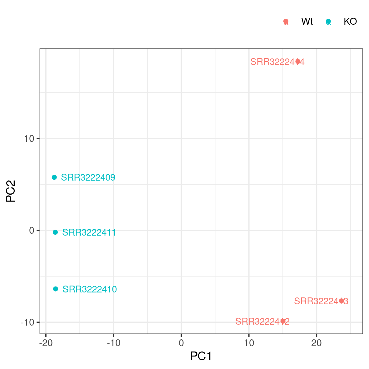
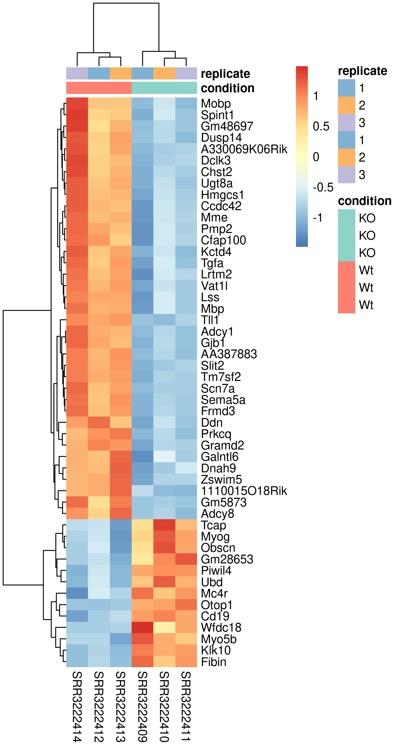
-rw-rw-r-- 1 user gXXXXXXX 1.7M Jan 22 23:16 dge_results_full.txtEssentially, we have two outputs: dge_results_full and counts_vst_full. dge_results_full is the list of differentially expressed genes. This is available in human readable tab-delimited .txt file and R readable binary .Rds file. The counts_vst_full is variance-stabilised normalised counts, useful for exploratory analyses.
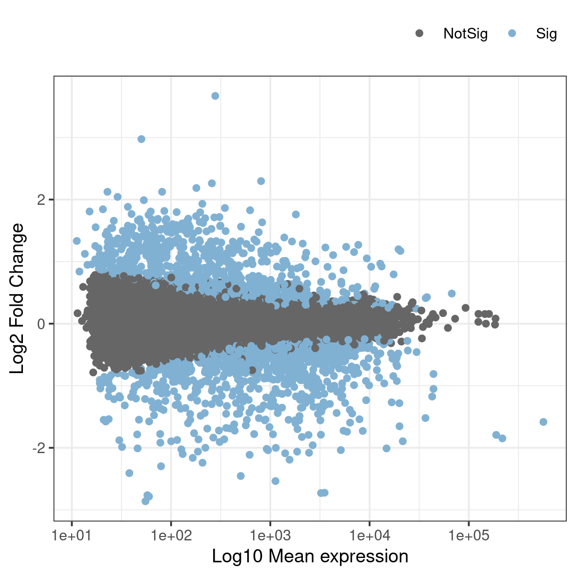
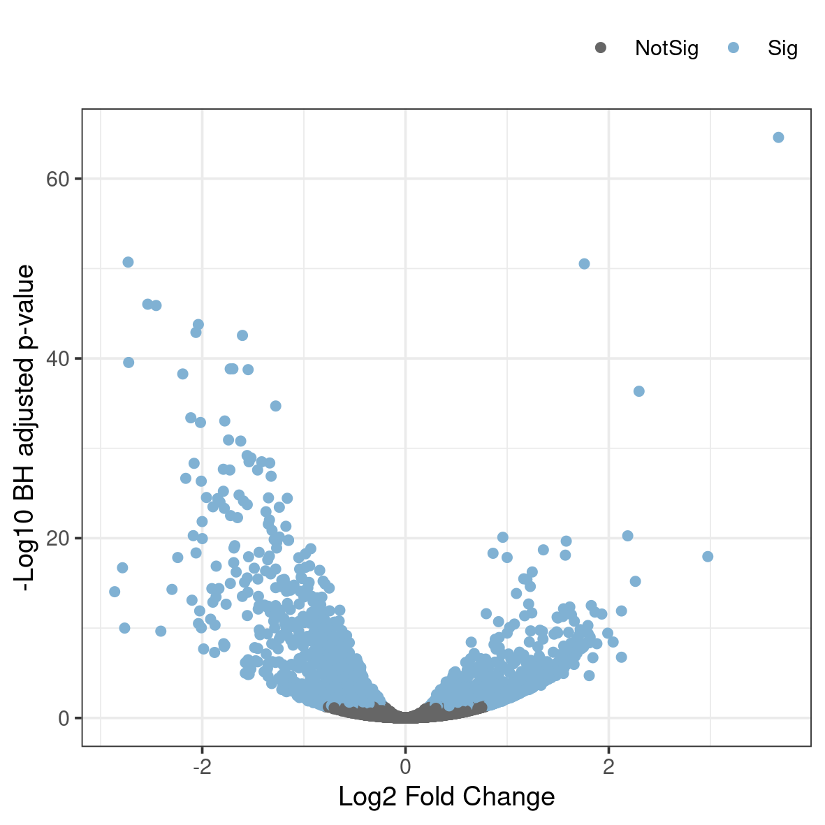
Copy the results text file (dge_results_full.txt) to your computer and inspect the results. What are the columns? How many differentially expressed genes are present after adjusted p-value of 0.05? How many genes are upregulated and how many are down-regulated? How does this change if we set a fold-change cut-off of 1?
Open in a spreadsheet editor like Microsoft Excel or LibreOffice Calc.
If you do not have the results or were unable to run the DGE step, you can copy these two here which will be required for functional annotation (optional).
cp /sw/courses/ngsintro/rnaseq/main/5_dge/dge_results_full.txt .
cp /sw/courses/ngsintro/rnaseq/main/5_dge/dge_results_full.Rds .
cp /sw/courses/ngsintro/rnaseq/main/5_dge/counts_vst_full.txt .
cp /sw/courses/ngsintro/rnaseq/main/5_dge/counts_vst_full.Rds .