Exercises: Discrete random variables

Introduction to probability

Exercise 1 (BRCA) The probability of carrying mutations (one or more) in the breast cancer gene BRCA1 is 0.01. What is the probability of not carrying any mutations in BRCA1?

Use the rule of complement.

According to the rule of complement \(P(no\,mutation) = 1 - P(mutations) = 1 - 0.01 = 0.99\)

Exercise 2 (A coin toss) When tossing a fair coin

  1. what is the probability of heads?
  2. what is the probability of tails?

Fair = equal probabilities

For a fair coin the probability of heads and tails are equal; \(P(H) = P(T)\). According to the rule of complement \(p(H) = 1 - P(T)\)

It follows that

  1. \(P(H) = 0.5\)
  2. \(P(T) = 0.5\)

Exercise 3 (Number of children) In a region in Sweden with many children the number of children per household is between 0 and 6. The probability mass function is as follows;

x 0 1 2 3 4 5 6
p(x) 0.14 0.20 0.27 0.19 0.13 0.05 0.02

In a randomly choosen household

  1. what is the probability of exactly 3 children?
  2. what is the probability of less than 3 children?
  3. what is the probability of 3 or less children?
  4. what is the probability of an even number of children?

In your answers, denote the probability with a mathematical expression (such as \(P(X>4)\)) and calculate its value.

The number of children in a random household is a random variable. Let \(X\) (a random variable) denote the number of children in a household in the studied region.

  1. \(P(X=3) = 0.19\)
  2. \(P(X<3) = P(X=0) + P(X=1) + P(X=2) = 0.14 + 0.20 + 0.27 = 0.61\)
  3. \(P(X \leq 3) = P(X=3) + P(X<3) = 0.19 + 0.61 = 0.80\)
  4. \(P(even\,X) = P(X=0) + P(X=2) + P(X=4) + P(X=6) = 0.14 + 0.27 + 0.13 + 0.02 = 0.56\)

Exercise 4 (Rolling dice) When tossing a fair six-sided dice

  1. what is the probability of getting 6?
  2. what is the probability of an even number?
  3. what is the probability of getting 3 or more?
  4. what is the expected value of dots on the dice?

On fair sided dice, all six sides have equal pobability.

The random variable, \(X\), describe the number of dots on the upper face of a dice.

  1. \(P(X=6) = \frac{1}{6}\)
  2. \(P(even\, X) = \frac{3}{6} = \frac{1}{2}\)
  3. \(P(X \geq 3) = \frac{4}{6} = \frac{2}{3}\)
  4. \(E[X] = 1*\frac{1}{6} + 2*\frac{1}{6} + 3*\frac{1}{6} + 4*\frac{1}{6} + 5*\frac{1}{6} + 6*\frac{1}{6} = 3.5\)

Simulation

Exercise 5 (Randomization) In a clinical trial, enrolled patients are randomly assigned to treatment or control group with equal probability.

For a single patient, what is the probability of being assigned to

  1. the treatment group?
  2. the control group?

If 20 patients are enrolled in the study;

  1. what is the probability of exactly 15 in the treatment group?
  2. what is the probability of less than 7 in the treatment group?
  3. What is the most probable number of patients in the treatment group?
  4. what is the probability of 5 or less patients in the control group?
  5. what is the probability of 2 or less patients in the treatment group?
  1. \(P(T)=0.5\)
  2. \(P(C) = 0.5\)
  1. The probability of assigning to control (C) and treatment (T) group are equal and sum up to 1. Hence \(P(T) = 0.5\) and;

  2. \(P(C) = 0.5\)

Simulate the assignment of patients into T or C groups.

## Randomization for a single patient
sample(c("T", "C"), size=1)
[1] "C"
## Randomize 20 independent patients
(patients <- sample(c("T", "c"), size=20, replace=TRUE))
 [1] "c" "T" "T" "c" "c" "c" "c" "T" "c" "T" "T" "c" "c" "T" "T" "c" "T" "T" "c"
[20] "T"
## How many patients are assigned to treatment group?
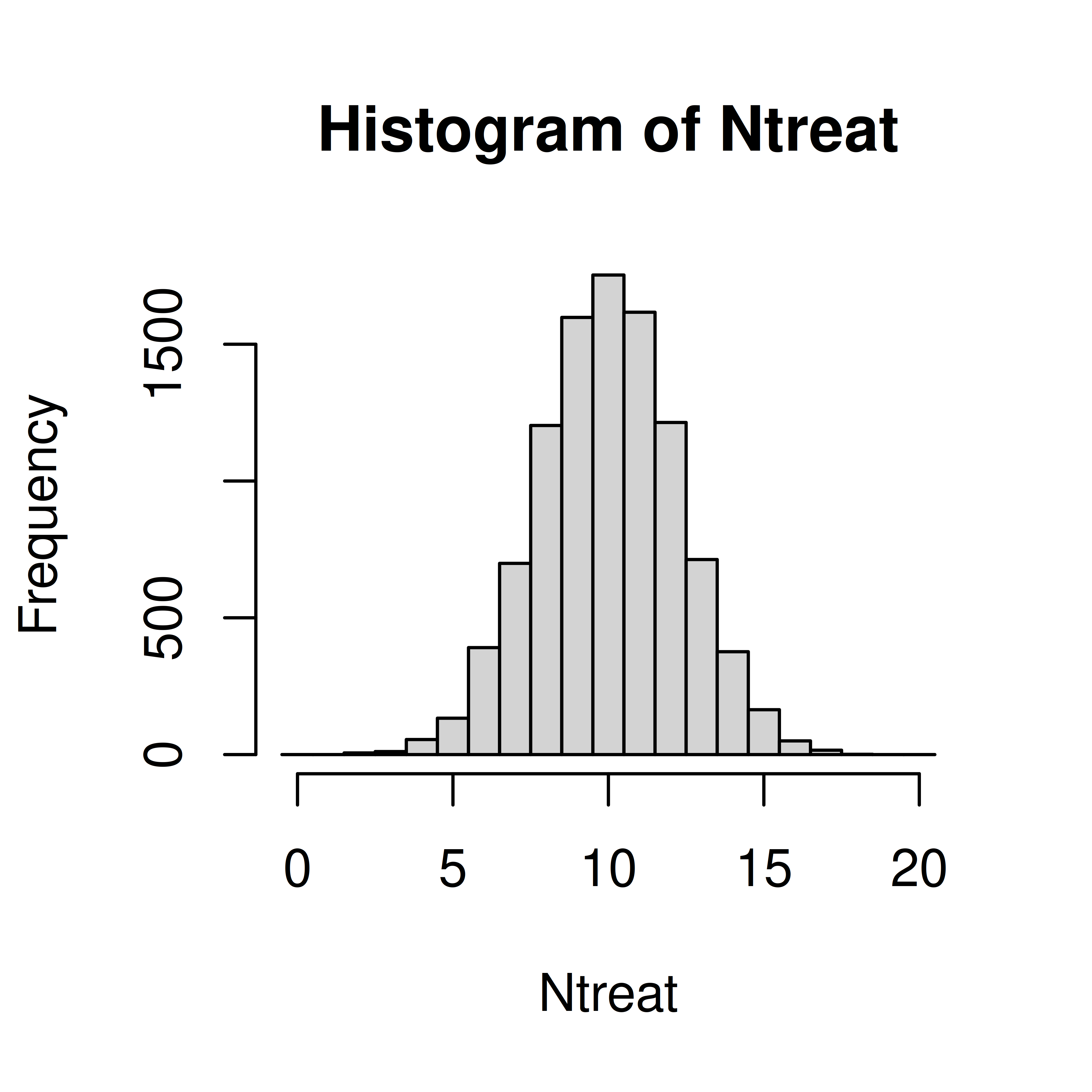
sum(patients == "T")
[1] 10
## Simulate by repeating 10000 times
Ntreat <- replicate(10000, {
  patients <- sample(c("T", "C"), size=20, replace=TRUE)
  sum(patients == "T")
})
  1. Probability of exactly 15 T
## Proportion of the 10000 repeats with exactly 15 T
mean(Ntreat==15)
[1] 0.016
  1. Probability of less than 7 T
mean(Ntreat<7)
[1] 0.06
  1. What is the most probable number of T patients?
## plot the distribution and read the graph
hist(Ntreat, breaks=0:21-0.5)

## or tabulate
table(Ntreat)
Ntreat
   2    3    4    5    6    7    8    9   10   11   12   13   14   15   16   17 
   6   11   55  133  391  699 1203 1598 1753 1617 1214  713  376  164   50   16 
  18 
   1 
  1. What is the probability of 5 C or less?

To get five or less C out of 20 throws is equal to getting 15 or more T out of 20.

## probability of 15 T or more
mean(Ntreat>=15)
[1] 0.023
  1. what is the probability of 2 T or less?
mean(Ntreat<=2)
[1] 6e-04
sum(Ntreat<=2)
[1] 6
## with this low number of observations, more repeats is required to get a more accurate answer
  
Ntreat <- replicate(1000000, {
  patients <- sample(c("T", "C"), size=20, replace=TRUE)
  sum(patients == "T")
})
sum(Ntreat<=2)
[1] 196
mean(Ntreat<=2)
[1] 2e-04

Exercise 6 (Bacterial colonies) In a bacterial sample, 1/6 are antibiotic resistant. From bacterial colonies on an agar plate, you randomly pick 10 colonies and investigate how many that are antibiotic resistant.

  1. Define the random variable of interest
  2. What are the possible outcomes?
  3. Using simulation, estimate the probability mass function
  4. what is the probability to get at least 5 antibiotic resistant colonies?
  5. Which is the most likely number of antibioitic colonies?
  6. What is the probability to get exactly 2 antibiotic resistant colonies?
  7. On average how many antibiotic resistant colonies would you get if the experiment is repeated many time?

Think of the dice example, where the probability of getting ‘six’ on one dice is 1/6.

  1. \(X\), the number of antibiotic resistant colonies out of 10.

  2. \({0, 1, 2, 3, 4, 5, 6, 7, 8, 9, 10}\)

##Simulate picking 10 colonies and counting the number of antibiotic resistant ones.
N <- replicate(100000, sum(sample(1:6, size=10, replace=TRUE)==6))
table(N)
N
    0     1     2     3     4     5     6     7     8 
16390 32371 29043 15314  5364  1268   224    24     2 
##The probability mass function
table(N)/length(N)
N
      0       1       2       3       4       5       6       7       8 
0.16390 0.32371 0.29043 0.15314 0.05364 0.01268 0.00224 0.00024 0.00002 
hist(N, breaks=(0:11)-0.5)

  1. 0.015
[1] 1518
[1] 0.015
[1] 0.015
  1. 1 (Use the PMF to answer this question)

  2. 0.29

mean(N==2)
[1] 0.29
  1. 1.7
mean(N)
[1] 1.7
10*1/6
[1] 1.7

Exercise 7 (Pollen allergy)  

  1. 30% of a large population is allergic to pollen. If you randomly select 3 people to participate in your study, what is the probability than none of them will be allergic to pollen?
## Solution using 100 replicates
x <- replicate(100, sum(sample(c(0,0,0,0,0,0,0,1,1,1), size=3, replace=TRUE)))
table(x)
x
 0  1  2  3 
38 42 18  2 
mean(x==0)
[1] 0.38
## Solution using 1000 replicates
x <- replicate(1000, sum(sample(c(0,0,0,0,0,0,0,1,1,1), size=3, replace=TRUE)))
table(x)
x
  0   1   2   3 
330 467 184  19 
mean(x==0)
[1] 0.33
## Solution using 100000 replicates
x <- replicate(100000, sum(sample(c(0,0,0,0,0,0,0,1,1,1), size=3, replace=TRUE)))
table(x)
x
    0     1     2     3 
34549 43850 19021  2580 
mean(x==0)
[1] 0.35
  1. In a class of 20 students, 6 are allergic to pollen. If you randomly select 3 of the students to participate in your study, what is the probability than none of them will be allergic to pollen?
## Solution using 100000 replicates
x <- replicate(100000, sum(sample(rep(c(0, 1), c(14, 6)), size=3, replace=FALSE)))
table(x)
x
    0     1     2     3 
32006 47761 18462  1771 
mean(x==0)
[1] 0.32
  1. Of the 200 persons working at a company, 60 are allergic to pollen. If you randomly select 3 people to participate in your study, what is the probability that none of them are allergic to pollen?
## Solution using 100000 replicates
x <- replicate(100000, sum(sample(rep(c(0, 1), c(140, 60)), size=3, replace=FALSE)))
table(x)
x
    0     1     2     3 
33896 44637 18820  2647 
mean(x==0)
[1] 0.34
  1. Compare your results in a, b and c. Did you get the same results? Why/why not?

The results differ. In a the probability of selecting an allergic person is constant, regardless of the status of previously selected persons. On the other hand in the situations in b and c, the probability of selecting an allergic person changes depending on the persons selected before.

Parametric discrete distribution

Exercise 8 (Pollen) Do Exercise 7 again, but using parametric distributions. Compare your results.

## 1.6 Solution using the Binomial distribution
pbinom(0, 3, 0.3)
[1] 0.34
## 1.7 Solution using the hypergeometric distribution
phyper(0, 6, 20-6, 3)
[1] 0.32
## 1.8 Solution using the hypergeometric distribution
phyper(0, 60, 200-60, 3)
[1] 0.34

Exercise 9 (Gene set enrichment analysis) You have analyzed 20000 genes and a bioinformatician you are collaborating with has sent you a list of 1000 genes that she says are important. You are interested in a particular pathway A. 200 genes in pathway A are represented among the 20000 genes, 20 of these are in the bioinformaticians important list.

If the bioinformatician selected the 1000 genes at random, what is the probability to see 20 or more genes from pathway A in this list?

phyper(20, 200, 20000-200, 1000, lower.tail=FALSE)
[1] 0.0011

Exercise 10 (Chance of meeting boss) Your boss comes in to the office three days per week. You do also come in to work three days per week. If you both choose which days to come in to work at random, what is the probability that a particular week you are in the office at the same time 0, 1, 2 or 3 days, respectively?

x <- replicate(100000, {x<-sample(1:5, 3); y<-sample(1:5,3); length(intersect(x,y))})
table(x)
x
    1     2     3 
29948 60038 10014 
dhyper(0:3, 3, 2, 3)
[1] 0.0 0.3 0.6 0.1

Exercise 11 (Rare disease) A rare disease affects 3 in 100000 in a large population. If 10000 people are randomly selected from the population, what is the probability

  1. that no one in the sample is affected?
  2. that at least two in the sample are affected?
n <- 10000
p <- 3/100000
ppois(0, n*p)
[1] 0.74
ppois(1, n*p, lower.tail=FALSE)
[1] 0.037