# create data recipe (feature engineering)
inch2m <- 2.54/100
pound2kg <- 0.45
data_recipe <- recipe(BMI ~ ., data = data_other) %>%
update_role(id, new_role = "sampleID") %>%
step_mutate(height = height * inch2m, height = round(height, 2)) %>% # convert height to meters
step_mutate(weight = weight * pound2kg, weight = round(weight, 2)) %>% # convert weight to kg
step_rename(glu = stab.glu) %>% # rename stab.glu to glu
step_log(glu) %>% #ln transform glucose
step_zv(all_numeric()) %>% # removes variables that are highly sparse and unbalanced (if found)
step_corr(all_numeric(), -all_outcomes(), -has_role("sampleID"), threshold = 0.8) %>% # removes variables with large absolute correlations with other variables (if found)
step_dummy(location, gender, frame) %>% # convert categorical variables to dummy variables
step_normalize(all_numeric(), -all_outcomes(), -has_role("sampleID"), skip = FALSE)
# you can implement more steps: see https://recipes.tidymodels.org/reference/index.html
# print recipe
data_recipe
# check if recipe is doing what it is supposed to do
# i.e. bake the data
data_other_prep <- data_recipe %>%
prep() %>%
bake(new_data = NULL)
## bake test data
data_test_prep <- data_recipe %>%
prep() %>%
bake(new_data = data_test)
# preview baked data
print(head(data_other_prep))
## # A tibble: 6 × 17
## id chol glu hdl ratio glyhb age height bp.1s bp.1d hip
## <dbl> <dbl> <dbl> <dbl> <dbl> <dbl> <dbl> <dbl> <dbl> <dbl> <dbl>
## 1 1045 -0.319 -0.539 -0.830 0.486 -0.172 -0.645 -0.474 -1.16 -0.552 -1.66
## 2 1271 0.449 -1.09 -0.324 0.320 -0.458 -1.39 -1.29 -1.59 -1.00 -0.914
## 3 1277 -0.657 -0.572 2.32 -1.45 -0.642 -0.337 1.56 0.286 2.15 -1.29
## 4 1303 -0.590 -0.410 -0.436 -0.178 -0.518 0.341 0.545 -0.309 0.500 -1.47
## 5 1309 -0.206 -0.347 0.687 -0.730 -0.860 -1.32 0.0357 -0.735 -0.402 -1.66
## 6 1315 -0.793 -0.572 0.350 -0.841 0.225 0.649 1.26 -0.565 -1.45 -1.29
## # … with 6 more variables: time.ppn <dbl>, BMI <dbl>, location_Louisa <dbl>,
## # gender_male <dbl>, frame_medium <dbl>, frame_small <dbl>2 Demo: a predictive modelling case study
Let’s use tidymodels framework to run small predictive case study trying to build a predictive model for BMI using our diabetes data set. We will use:
rsamplesfor splitting data into test and non-test, as well as creating cross-validation foldsrecipesfor feature engineering, e.g. changing from imperial to metric measurements, removing irrelevant and highly correlated featuresparsnipto specify Lasso regression modeltuneto optimize search space for lambda valuesyardstickto assess predictionsworkflowsto put all the step together
2.1 Data import & EDA
# load libraries
library(tidyverse)
library(tidymodels)
library(ggcorrplot)
library(reshape2)
library(vip)

# import raw data
input_diabetes <- read_csv("data/data-diabetes.csv")

# create BMI variable
conv_factor <- 703 # conversion factor to calculate BMI from inches and pounds BMI = weight (lb) / [height (in)]2 x 703
data_diabetes <- input_diabetes %>%
  mutate(BMI = weight / height^2 * 703, BMI = round(BMI, 2)) %>%
  relocate(BMI, .after = id)

# preview data
glimpse(data_diabetes)
## Rows: 403
## Columns: 20
## $ id       <dbl> 1000, 1001, 1002, 1003, 1005, 1008, 1011, 1015, 1016, 1022, 1…
## $ BMI      <dbl> 22.13, 37.42, 48.37, 18.64, 27.82, 26.50, 28.20, 34.33, 24.51…
## $ chol     <dbl> 203, 165, 228, 78, 249, 248, 195, 227, 177, 263, 242, 215, 23…
## $ stab.glu <dbl> 82, 97, 92, 93, 90, 94, 92, 75, 87, 89, 82, 128, 75, 79, 76, …
## $ hdl      <dbl> 56, 24, 37, 12, 28, 69, 41, 44, 49, 40, 54, 34, 36, 46, 30, 4…
## $ ratio    <dbl> 3.6, 6.9, 6.2, 6.5, 8.9, 3.6, 4.8, 5.2, 3.6, 6.6, 4.5, 6.3, 6…
## $ glyhb    <dbl> 4.31, 4.44, 4.64, 4.63, 7.72, 4.81, 4.84, 3.94, 4.84, 5.78, 4…
## $ location <chr> "Buckingham", "Buckingham", "Buckingham", "Buckingham", "Buck…
## $ age      <dbl> 46, 29, 58, 67, 64, 34, 30, 37, 45, 55, 60, 38, 27, 40, 36, 3…
## $ gender   <chr> "female", "female", "female", "male", "male", "male", "male",…
## $ height   <dbl> 62, 64, 61, 67, 68, 71, 69, 59, 69, 63, 65, 58, 60, 59, 69, 6…
## $ weight   <dbl> 121, 218, 256, 119, 183, 190, 191, 170, 166, 202, 156, 195, 1…
## $ frame    <chr> "medium", "large", "large", "large", "medium", "large", "medi…
## $ bp.1s    <dbl> 118, 112, 190, 110, 138, 132, 161, NA, 160, 108, 130, 102, 13…
## $ bp.1d    <dbl> 59, 68, 92, 50, 80, 86, 112, NA, 80, 72, 90, 68, 80, NA, 66, …
## $ bp.2s    <dbl> NA, NA, 185, NA, NA, NA, 161, NA, 128, NA, 130, NA, NA, NA, N…
## $ bp.2d    <dbl> NA, NA, 92, NA, NA, NA, 112, NA, 86, NA, 90, NA, NA, NA, NA, …
## $ waist    <dbl> 29, 46, 49, 33, 44, 36, 46, 34, 34, 45, 39, 42, 35, 37, 36, 3…
## $ hip      <dbl> 38, 48, 57, 38, 41, 42, 49, 39, 40, 50, 45, 50, 41, 43, 40, 4…
## $ time.ppn <dbl> 720, 360, 180, 480, 300, 195, 720, 1020, 300, 240, 300, 90, 7…

# run basic EDA
# note: we have seen descriptive statistics and plots during EDA session
# note: so here we only look at missing data and correlation

# calculate number of missing data per variable
data_na <- data_diabetes %>%
  summarise(across(everything(), ~ sum(is.na(.))))

# make a table with counts sorted from highest to lowest
data_na_long <- data_na %>%
  pivot_longer(-id, names_to = "variable", values_to = "count") %>%
  arrange(desc(count))

# make a column plot to visualize the counts
data_na_long %>%
  ggplot(aes(x = variable, y = count)) +
  geom_col(fill = "blue4") +
  xlab("") +
  theme_bw() +
  theme(axis.text.x = element_text(angle = 45, vjust = 1, hjust=1))

# calculate correlation between numeric variables
data_cor <- data_diabetes %>%
  dplyr::select(-id) %>%
  dplyr::select(where(is.numeric)) %>%
  cor(use = "pairwise.complete.obs")

# visualize correlation via heatmap
ggcorrplot(data_cor, hc.order = TRUE, lab = FALSE)

# bass on the number of missing data, let's delete bp.2s, bp.2d
# and use complete-cases analysis
data_diabetes_narm <- data_diabetes %>%
  dplyr::select(-bp.2s, -bp.2d) %>%
  na.omit()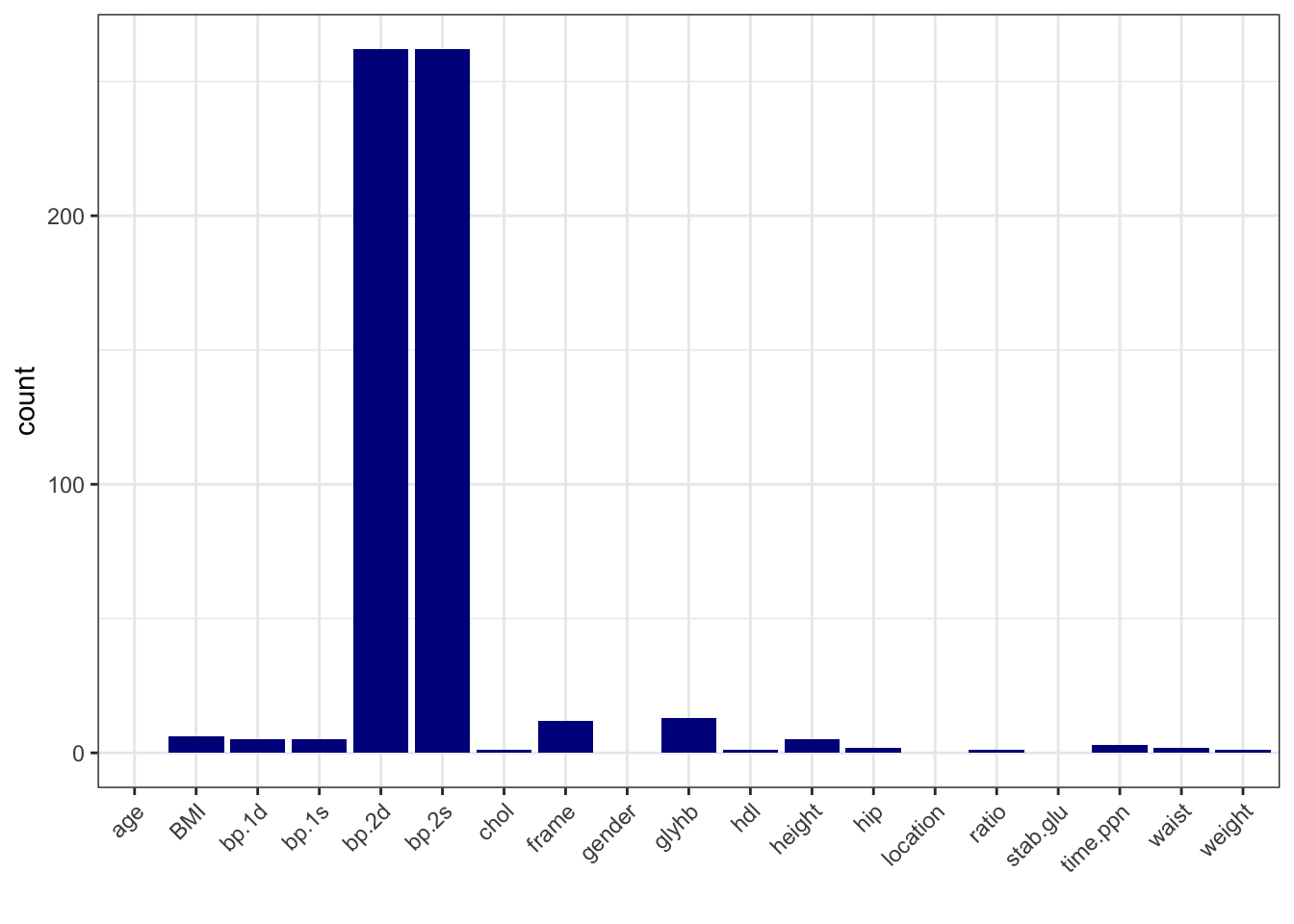

2.2 Data splitting
# use tidymodels framework to fit Lasso regression model for predicting BMI
# using repeated cross-validation to tune lambda value in L1 penalty term

# select random seed value
myseed <- 123

# split data into non-test (other) and test (80% s)
set.seed(myseed)
data_split <- initial_split(data_diabetes_narm, strata = BMI, prop = 0.8) # holds splitting info
data_other <- data_split %>% training() # creates non-test set (function is called training but it refers to non-test part)
data_test <- data_split %>% testing() # creates test set

# prepare repeated cross-validation splits with 5 folds repeated 3 times
set.seed(myseed)
data_folds <- vfold_cv(data_other,
                       v = 5,
                       repeats = 3,
                       strata = BMI)

# check the split
dim(data_diabetes)
## [1] 403  20
dim(data_other)
## [1] 291  18
dim(data_test)
## [1] 75 18

# check BMI distributions in data splits
par(mfrow=c(3,1))
hist(data_diabetes$BMI, xlab = "", main = "BMI: all", 50)
hist(data_other$BMI, xlab = "", main = "BMI: non-test", 50)
hist(data_test$BMI, xlab = "", main = "BMI: test", 50)
2.3 Feature engineering
2.4 Lasso regression
# define model
model <- linear_reg(penalty = tune(), mixture = 1) %>%
set_engine("glmnet") %>%
set_mode("regression")
# create workflow with data recipe and model
wf <- workflow() %>%
add_model(model) %>%
add_recipe(data_recipe)
# define parameters range for tuning
grid_lambda <- grid_regular(penalty(), levels = 25)
# tune lambda
model_tune <- wf %>%
tune_grid(resamples = data_folds,
grid = grid_lambda)
# show metrics average across folds
model_tune %>%
collect_metrics(summarize = TRUE)
## # A tibble: 50 × 7
## penalty .metric .estimator mean n std_err .config
## <dbl> <chr> <chr> <dbl> <int> <dbl> <chr>
## 1 1 e-10 rmse standard 2.48 15 0.142 Preprocessor1_Model01
## 2 1 e-10 rsq standard 0.851 15 0.0143 Preprocessor1_Model01
## 3 2.61e-10 rmse standard 2.48 15 0.142 Preprocessor1_Model02
## 4 2.61e-10 rsq standard 0.851 15 0.0143 Preprocessor1_Model02
## 5 6.81e-10 rmse standard 2.48 15 0.142 Preprocessor1_Model03
## 6 6.81e-10 rsq standard 0.851 15 0.0143 Preprocessor1_Model03
## 7 1.78e- 9 rmse standard 2.48 15 0.142 Preprocessor1_Model04
## 8 1.78e- 9 rsq standard 0.851 15 0.0143 Preprocessor1_Model04
## 9 4.64e- 9 rmse standard 2.48 15 0.142 Preprocessor1_Model05
## 10 4.64e- 9 rsq standard 0.851 15 0.0143 Preprocessor1_Model05
## # … with 40 more rows
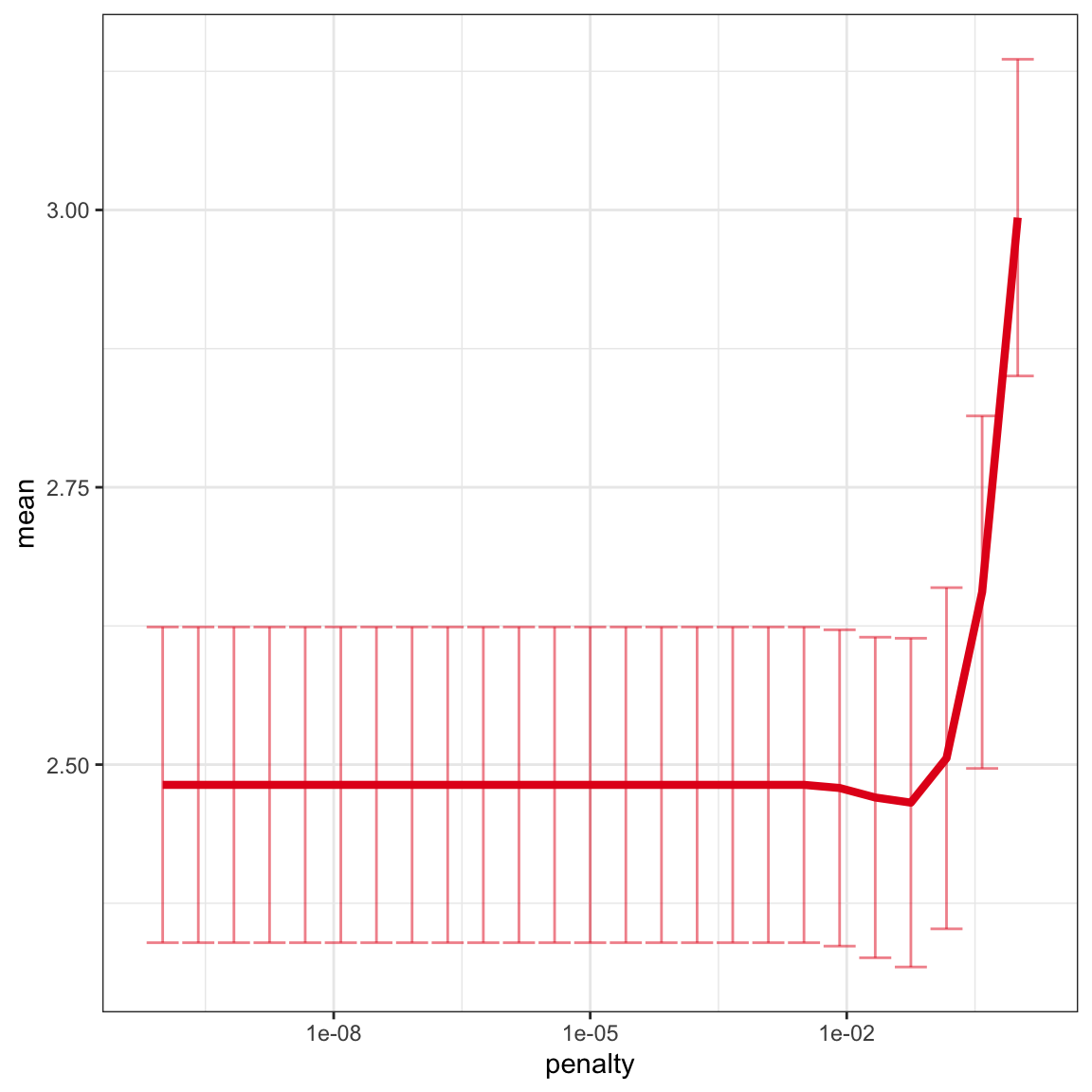
# plot k-folds results across lambda range
model_tune %>%
collect_metrics() %>%
dplyr::filter(.metric == "rmse") %>%
ggplot(aes(penalty, mean, color = .metric)) +
geom_errorbar(aes( ymin = mean - std_err, ymax = mean + std_err), alpha = 0.5) +
scale_x_log10() +
geom_line(linewidth = 1.5) +
theme_bw() +
theme(legend.position = "none") +
scale_color_brewer(palette = "Set1")
# best lambda value (min. RMSE)
model_best <- model_tune %>%
select_best("rmse")
print(model_best)
## # A tibble: 1 × 2
## penalty .config
## <dbl> <chr>
## 1 0.0562 Preprocessor1_Model22
# finalize workflow with tuned model
wf_final <- wf %>%
finalize_workflow(model_best)
# last fit
fit_final <- wf_final %>%
last_fit(split = data_split)
# final predictions
y_test_pred <- fit_final %>% collect_predictions() # predicted BMI
# final predictions: performance on test (unseen data)
fit_final %>% collect_metrics()
## # A tibble: 2 × 4
## .metric .estimator .estimate .config
## <chr> <chr> <dbl> <chr>
## 1 rmse standard 2.79 Preprocessor1_Model1
## 2 rsq standard 0.857 Preprocessor1_Model1
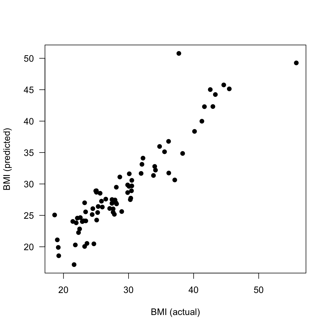
# plot predictions vs. actual for test data
plot(data_test$BMI, y_test_pred$.pred, xlab="BMI (actual)", ylab = "BMI (predicted)", las = 1, pch = 19)
# correlation between predicted and actual BMI values for test data
cor(data_test$BMI, y_test_pred$.pred)
## [1] 0.9256857
# re-fit model on all non-test data
model_final <- wf_final %>%
fit(data_other)
# show final model
tidy(model_final)
## # A tibble: 16 × 3
## term estimate penalty
## <chr> <dbl> <dbl>
## 1 (Intercept) 28.7 0.0562
## 2 chol 0 0.0562
## 3 glu 0.0229 0.0562
## 4 hdl 0 0.0562
## 5 ratio 0.335 0.0562
## 6 glyhb -0.0512 0.0562
## 7 age -0.257 0.0562
## 8 height -1.86 0.0562
## 9 bp.1s -0.294 0.0562
## 10 bp.1d 0.203 0.0562
## 11 hip 5.60 0.0562
## 12 time.ppn 0 0.0562
## 13 location_Louisa -0.160 0.0562
## 14 gender_male 1.07 0.0562
## 15 frame_medium -0.320 0.0562
## 16 frame_small -0.530 0.0562
# plot variables ordered by importance (highest abs(coeff))
model_final %>%
extract_fit_parsnip() %>%
vip(geom = "point") +
theme_bw()