Bagging, boosting and stacking

Introduction

We are still working to better understand the biology of obesity. Previous studies have shown that the expression of several genes (FTO, MC4R, LEP) is associated with this condition. In this exercise, we are interested in building a predictive model for obesity based on gene expression data, focusing on less well-known genes.

We will explore three ensemble learning strategies:

Bagging, using Random Forest;
Boosting, using XGBoost;
Stacking, combining the predictions from KNN, SVM, and Random Forest, with logistic regression as a meta-learner.

Load packages

Code

# load packages
rm(list=ls())
library(tidyverse)
library(ggcorrplot)
library(glmnet)
library(fastDummies)
library(pROC)
library(ranger)
library(e1071)
library(class)
library(xgboost)

# Load the clinical data
data_obesity <- read_csv("data/data-obesity.csv") 

# Load gene expression data
data_expr <- read_csv("data/data-obesity-genes.csv")
genes_all <- colnames(data_expr)[-1]  # Exclude the 'id' column

# Genes
gens_known <- c("FTO", "MC4R", "LEP")
genes_other <- setdiff(genes_all, gens_known)

Split Data

# join gene expression data with clinical data
data <- data_obesity %>%
  left_join(data_expr, by = "id") %>%
  dplyr::select("obese", all_of(genes_other)) %>%
  na.omit()

# three-way split: train (60%), validation (20%), test (20%)
set.seed(123)
n <- nrow(data)
idx <- sample(seq_len(n))
idx_train <- idx[1:floor(0.6 * n)]
idx_valid <- idx[(floor(0.6 * n) + 1):floor(0.8 * n)]
idx_test  <- idx[(floor(0.8 * n) + 1):n]

data_train <- data[idx_train, ]
data_valid <- data[idx_valid, ]
data_test  <- data[idx_test, ]

# To keep focus on the important parts, we will skip feature engineering
# and we will just scale all data
x_train <- data_train %>%
  dplyr::select(-obese) %>%
  as.matrix() %>%
  scale()

x_valid <- data_valid %>%
  dplyr::select(-obese) %>%
  as.matrix() %>%
  scale()

x_test <- data_test %>%
  dplyr::select(-obese) %>%
  as.matrix() %>%
  scale()

# Separate and format target variable
y_train <- data_train$obese
y_train <- ifelse(y_train == "Yes", 1, 0) 

y_valid <- data_valid$obese
y_valid <- ifelse(y_valid == "Yes", 1, 0)

y_test <- data_test$obese
y_test <- ifelse(y_test == "Yes", 1, 0)

Bagging: Random Forest

Code


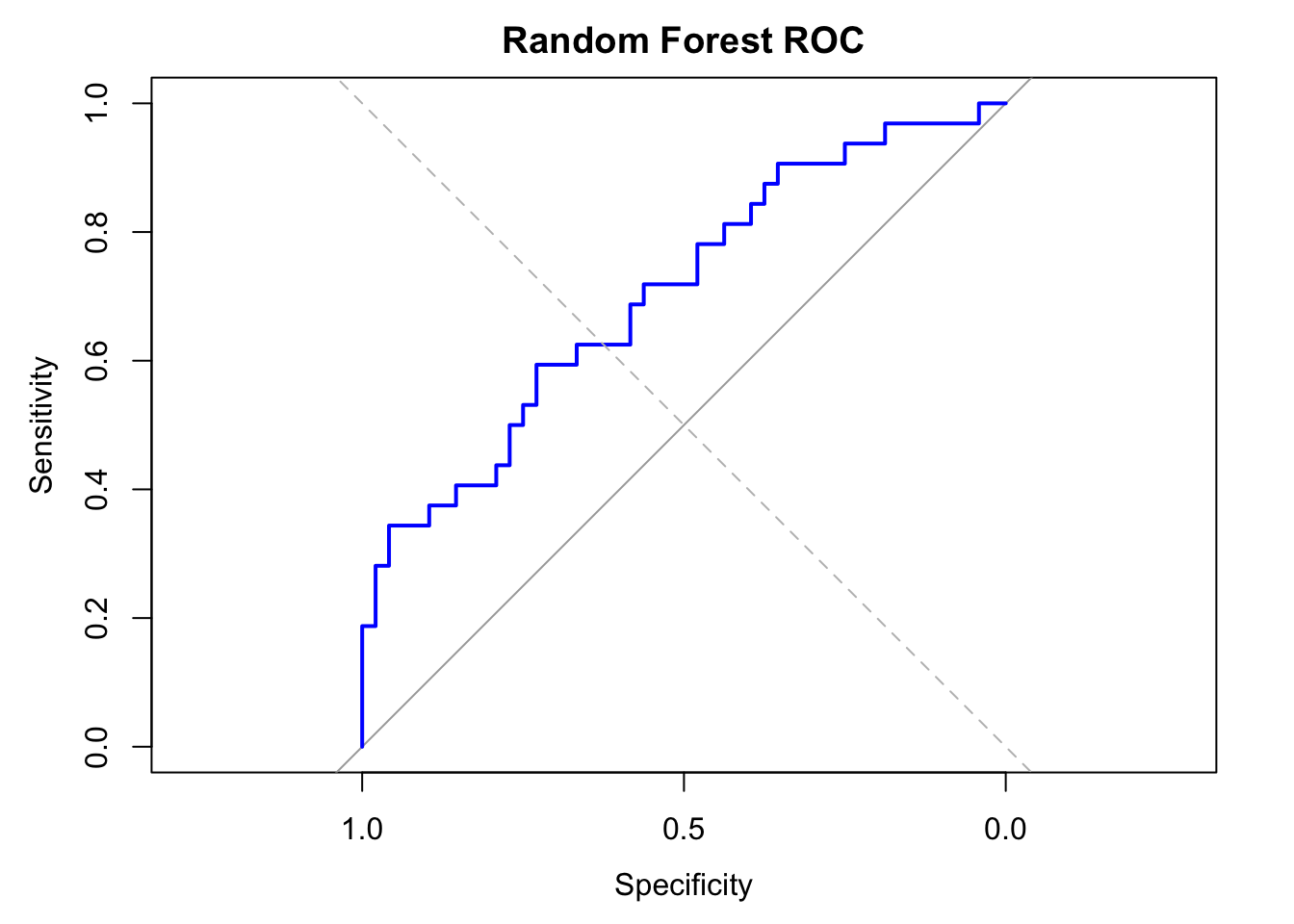
# Combine predictors and target into a single data frame for ranger
df_train <- data.frame(y = factor(data_train$obese), x_train)
df_valid <- data.frame(y = factor(data_valid$obese), x_valid)
df_test <- data.frame(y = factor(data_test$obese), x_test)

# Tune RF
# Grid search over mtry and min.node.size
results <- expand.grid(
  mtry = c(5, 10, 20, 50),
  min.node.size = c(1, 5, 10)
)

# Create a function to evaluate AUC for a set of parameters
tune_rf <- function(mtry_val, min_node) {
  rf_model <- ranger(
    y ~ ., data = df_train,
    probability = TRUE,
    num.trees = 500,
    mtry = mtry_val,
    min.node.size = min_node,
    seed = 123
  )
  
  rf_probs <- predict(rf_model, data = df_valid)$predictions[, "Yes"]
  roc_obj <- roc(df_valid$y, rf_probs, quiet = TRUE)
  auc_val <- auc(roc_obj)
  return(auc_val)
}

results$AUC <- mapply(tune_rf, results$mtry, results$min.node.size)

# Find best combination
best_params <- results[which.max(results$AUC), ]
print(best_params)
##   mtry min.node.size       AUC
## 8   50             5 0.9024217

# Refit final tuned Random Forest model with best hyperparameters
rf_model <- ranger(
  y ~ ., data = df_train,
  probability = TRUE,
  num.trees = 500,
  mtry = best_params$mtry,
  min.node.size = best_params$min.node.size,
  seed = 123, 
  importance = "impurity"
)

# Predict and evaluate on test data
rf_probs <- predict(rf_model, data = df_test)$predictions[, "Yes"]
rf_preds <- ifelse(rf_probs > 0.5, "Yes", "No")

# Confusion matrix
conf_matrix <- table(Predicted = rf_preds, Actual = df_test$y)
print(conf_matrix)
##          Actual
## Predicted No Yes
##       No  48  28
##       Yes  0   4

# Accuracy and AUC
accuracy <- sum(diag(conf_matrix)) / sum(conf_matrix)
roc_obj <- roc(df_test$y, rf_probs)
auc_val <- auc(roc_obj)

plot(roc_obj, col = "blue", lwd = 2, main = "Random Forest ROC")
abline(a = 0, b = 1, lty = 2, col = "gray")
cat("AUC:", auc(roc_obj), "\n")
## AUC: 0.7044271

rf_conf_matrix <- conf_matrix
rf_acc <- accuracy
rf_auc <- auc_val

rf_best_parm <- best_params

cat(sprintf("Random Forest Test Accuracy: %.3f\n", rf_acc))
## Random Forest Test Accuracy: 0.650
cat(sprintf("Random Forest Test AUC: %.3f\n", rf_auc))
## Random Forest Test AUC: 0.704

Code

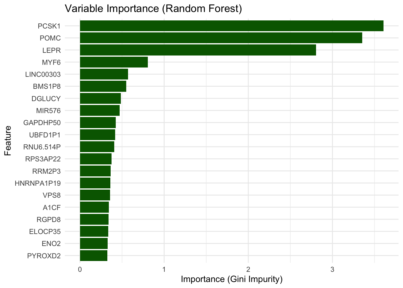
# feature importance
importance <- rf_model$variable.importance

# Convert to data frame
importance_df <- data.frame(
  feature = names(importance),
  importance = importance
)

# Plot top features
importance_df <- importance_df %>%
  arrange(desc(importance))

ggplot(importance_df[1:20, ], aes(x = reorder(feature, importance), y = importance)) +
  geom_col(fill = "darkgreen") +
  coord_flip() +
  labs(
    title = "Variable Importance (Random Forest)",
    x = "Feature", y = "Importance (Gini Impurity)"
  ) +
  theme_minimal()

Boosting: XGBoost

Code

# Prepare data
dtrain <- xgb.DMatrix(data = x_train, label = y_train)  
dvalid <- xgb.DMatrix(data = x_valid, label = y_valid)
dtest  <- xgb.DMatrix(data = x_test)

# Define parameter grid
xgb_grid <- expand.grid(
  eta = c(0.01, 0.1, 0.3),
  max_depth = c(3, 5, 7)
)

# Tuning loop
xgb_grid$AUC <- NA

for (i in 1:nrow(xgb_grid)) {
  params <- list(
    objective = "binary:logistic",
    eval_metric = "auc",
    eta = xgb_grid$eta[i],
    max_depth = xgb_grid$max_depth[i]
  )
  
  xgb_model <- xgb.train(
    params = params,
    data = dtrain,
    nrounds = 100,
    verbose = 0
  )
  
  valid_probs <- predict(xgb_model, newdata = dvalid)
  roc_obj <- roc(y_valid, valid_probs, quiet = TRUE)
  xgb_grid$AUC[i] <- auc(roc_obj)
}

# Best model
best_params <- xgb_grid[which.max(xgb_grid$AUC), ]
print(best_params)
##   eta max_depth       AUC
## 6 0.3         5 0.9009972

# Refit using best parameters
final_xgb <- xgb.train(
  params = list(
    objective = "binary:logistic",
    eval_metric = "auc",
    eta = best_params$eta,
    max_depth = best_params$max_depth
  ),
  data = dtrain,
  nrounds = 100,
  verbose = 0
)

# Test predictions
xgb_probs <- predict(final_xgb, newdata = dtest)
xgb_preds <- ifelse(xgb_probs > 0.5, "Yes", "No")

# Evaluation
xgb_conf_matrix <- table(Predicted = xgb_preds, Actual = y_test)
xgb_acc <- sum(diag(xgb_conf_matrix)) / sum(xgb_conf_matrix)
xgb_auc <- auc(roc(y_test, xgb_probs))

print(xgb_conf_matrix)
##          Actual
## Predicted  0  1
##       No  40 13
##       Yes  8 19
cat(sprintf("XGBoost Test Accuracy: %.3f\n", xgb_acc))
## XGBoost Test Accuracy: 0.738
cat(sprintf("XGBoost Test AUC: %.3f\n", xgb_auc))
## XGBoost Test AUC: 0.819

Stacking

Let’s combine the predictions from Random Forest, SVM and KNN models using a stacking ensemble approach. We will use logistic regression as the meta-model. We have already tuned Random Forest, so we will need to tune SVM and KNN before proceeding with stacking.

SVM

Code

# SVM with linear kernel

# Prepare data for SMV
data_train_svm <- data_train %>%
  mutate(obese = factor(obese, levels = c("No", "Yes")))

data_valid_svm <- data_valid %>%
  mutate(obese = factor(obese, levels = c("No", "Yes")))

# Try different cost values for SVM
cost_grid <- c(0.01, 0.1, 1, 10)
svm_results <- data.frame(cost = cost_grid, AUC = NA)

for (i in seq_along(cost_grid)) {
  
  model <- svm(obese ~ ., data = data_train_svm, cost = cost_grid[i], probability = TRUE)
  pred <- predict(model, newdata = data_valid_svm, probability = TRUE)
  probs <- attr(pred, "probabilities")[, "Yes"]
  svm_results$AUC[i] <- auc(roc(data_valid_svm$obese, probs, quiet = TRUE))
  
}

# Find the best cost value based on AUC
best_cost <- svm_results$cost[which.max(svm_results$AUC)]

# Fit the final SVM model with the best cost
svm_model <- svm(obese ~ ., data = data_train_svm, cost = best_cost, probability = TRUE)

# Predict on test sets
svm_test_pred <- predict(svm_model, newdata = data_test, probability = TRUE)
svm_test_probs <- attr(svm_test_pred, "probabilities")[, "Yes"]

# Accuracy and AUC for SVM
svm_preds <- ifelse(svm_test_probs > 0.5, "Yes", "No")
svm_acc <- mean(svm_preds == data_test$obese)
svm_auc <- auc(roc(data_test$obese, svm_test_probs, quiet = TRUE))

svm_best_cost <- best_cost

cat(sprintf("SVM Test Accuracy: %.3f\n", svm_acc))
## SVM Test Accuracy: 0.537
cat(sprintf("SVM Test AUC: %.3f\n", svm_auc))
## SVM Test AUC: 0.458

KNN

Code

# Tune KNN using validation AUC
k_values <- c(3, 5, 7, 9, 11, 13, 15)
knn_results <- data.frame(k = k_values, AUC = NA)

for (i in seq_along(k_values)) {
  
  pred <- knn(train = x_train, test = x_valid, cl = data_train$obese, k = k_values[i], prob = TRUE)
  probs <- ifelse(pred == "Yes", attr(pred, "prob"), 1 - attr(pred, "prob"))
  knn_results$AUC[i] <- auc(roc(data_valid$obese, probs, quiet = TRUE))
  
}

best_k <- knn_results$k[which.max(knn_results$AUC)]

# Fit the final KNN model with the best k
knn_test <- knn(train = x_train, test = x_test,
                cl = data_train$obese, k = best_k, prob = TRUE)
knn_test_probs <- ifelse(knn_test == "Yes", attr(knn_test, "prob"), 1 - attr(knn_test, "prob"))

# Accuracy and AUC for KNN
knn_preds <- ifelse(knn_test_probs > 0.5, "Yes", "No")
knn_acc <- mean(knn_preds == data_test$obese)
knn_auc <- auc(roc(data_test$obese, knn_test_probs, quiet = TRUE))

cat(sprintf("KNN Test Accuracy: %.3f\n", knn_acc))
## KNN Test Accuracy: 0.550
cat(sprintf("KNN Test AUC: %.3f\n", knn_auc))
## KNN Test AUC: 0.532

Stacking base models

The meta-learner is trained using the predicted probabilities from each base model (RF, SVM, KNN) on the validation set, learning how to best combine them.

Code

# Meta-learner is trained on validation-set predicted probabilities from each base model (RF, SVM, KNN)

# get validation probabilities for each tuned base model
rf_valid_probs <- predict(rf_model, data = df_valid)$predictions[, "Yes"]
svm_valid_probs <- predict(svm_model, newdata = data_valid_svm, probability = TRUE)
svm_valid_probs <- attr(svm_valid_probs, "probabilities")[, "Yes"]
knn_valid <- knn(train = x_train, test = x_valid,
                 cl = data_train$obese, k = best_k, prob = TRUE)
knn_valid_probs <- ifelse(knn_valid == "Yes", attr(knn_valid, "prob"), 1 - attr(knn_valid, "prob"))

# Combine validation predictions for meta-model
stack_valid <- data.frame(
  rf = rf_valid_probs,
  svm = svm_valid_probs,
  knn = knn_valid_probs,
  obese = as.factor(data_valid$obese)
)

x_meta <- model.matrix(obese ~ . - 1, data = stack_valid)
y_meta <- as.numeric(stack_valid$obese) - 1

# Combine test predictions for meta-model
stack_test <- data.frame(
  rf = predict(rf_model, data = df_test)$predictions[, "Yes"],
  svm = svm_test_probs,
  knn = knn_test_probs
)
x_stack_test <- model.matrix(~ . - 1, data = stack_test)

# Tune meta-model using Lasso regression
meta_model <- cv.glmnet(x_meta, y_meta, family = "binomial", alpha = 1)
best_lambda <- meta_model$lambda.min
cat("Best lambda:", best_lambda)
## Best lambda: 0.002781908

# Predict on test set using the meta-model
stack_probs <- predict(meta_model, newx = x_stack_test, s = "lambda.min", type = "response")
stack_preds <- ifelse(stack_probs > 0.5, "Yes", "No") |> factor(levels = c("No", "Yes"))

# Accuracy and AUC for stacked ensemble
stack_acc <- mean(stack_preds == data_test$obese)
stack_auc <- auc(roc(data_test$obese, as.numeric(stack_preds == "Yes"), quiet = TRUE))

Results

Code

# Create a results table
results_table <- data.frame(
  Model = c("Random Forest", "XGBoost", "SVM", "KNN", "Stacked"),
  Accuracy = c(rf_acc, xgb_acc, svm_acc, knn_acc, stack_acc),
  AUC = c(rf_auc, xgb_auc, svm_auc, knn_auc, stack_auc)
)

results_table <- results_table %>%
  mutate(Accuracy = round(Accuracy, 2),
         AUC = round(AUC, 2)) 

print(results_table)
##           Model Accuracy  AUC
## 1 Random Forest     0.65 0.70
## 2       XGBoost     0.74 0.82
## 3           SVM     0.54 0.46
## 4           KNN     0.55 0.53
## 5       Stacked     0.68 0.66

Comments:

GBoost is clearly the best performer, with the highest accuracy (0.74) and AUC (0.82), indicating strong predictive power and probability calibration.
Random Forest performs moderately, with decent AUC (0.70) but lower accuracy than XGBoost.
SVM and KNN underperform both in accuracy and AUC, suggesting they may not be well-suited for the structure of the gene expression data.
Stacked Ensemble improves upon Random Forest and the weaker base models, but does not outperform XGBoost, showing accuracy of 0.68 and AUC of 0.66.
This suggests stacking helped stabilize performance, but couldn’t exceed the strongest individual learner, possibly due to weak or correlated base model predictions.

To improve the stacking model, we could consider:

Adding more diverse models, e.g. including XGBoost, or LASSO logistic regression, to reduce redundancy among base learners.
Tuning the meta-learner more carefully by trying both lambda.min and lambda.1se for LASSO; or trying different meta-learner
Including raw features in the meta-learner, e.g by combining predicted probabilities with a few key original features (e.g., top gene expressions) to provide richer inputs.
Checking for prediction correlation: High correlation between base model outputs reduces the benefit of stacking—replace or drop highly redundant learners.
Trying alternative performance metrics, e.g. if our main main goal is identifying obese individuals, we could consider optimizing for recall, F1-score, instead of accuracy or AUC.

Task I

Experiment with the above suggestions, to see if you can improve the stacking model performance.

Task II

Modify the above code for a regression task, predicting BMI instead of obesity.