4 t-SNE and UMAP

4.1 Introduction

In this tutorial, we explore two popular nonlinear methods: t-SNE (t-distributed Stochastic Neighbor Embedding) and UMAP (Uniform Manifold Approximation and Projection).

4.2 t-SNE

t-SNE works by computing pairwise similarities between points in high-dimensional space, then finding a low-dimensional embedding that preserves those similarities. It minimizes the divergence between probability distributions using gradient descent. It is particularly good at keeping similar points close together.

Steps in t-SNE

Compute pairwise distances between all data points in high-dimensional space.
Convert distances to conditional probabilities representing similarities.
Initialize points randomly in 2D or 3D space.
Compute low-dimensional similarities using a t-distribution.
Minimize the Kullback-Leibler divergence between the two distributions using gradient descent.
Update points iteratively to reduce divergence.

4.3 UMAP

UMAP constructs a high-dimensional graph representing the data and then optimizes a low-dimensional projection that preserves both local neighborhoods and some global relationships. It is built on manifold learning and is generally faster than t-SNE, scaling better to large datasets.

Steps in UMAP

Compute k-nearest neighbors for each data point.
Estimate the probability graph based on local distances.
Construct a fuzzy topological representation of the data.
Initialize low-dimensional embedding randomly.
Optimize layout to preserve high-dimensional graph structure in low dimensions using stochastic gradient descent.

4.4 Data

library(tidyverse)
library(mixOmics)
data(breast.TCGA)

# Combine training and test sets
x <- rbind(breast.TCGA$data.train$mirna, breast.TCGA$data.test$mirna)
labels <- factor(c(breast.TCGA$data.train$subtype, breast.TCGA$data.test$subtype))

# Scale the data
x_scaled <- scale(x)

library(mixOmics)
data(breast.TCGA)

x <- rbind(breast.TCGA$data.train$mirna,breast.TCGA$data.test$mirna)
group_labels <-c(breast.TCGA$data.train$subtype,breast.TCGA$data.test$subtype)

# data dimensions
x |> dim() |> print () # dimensions of the data matrix (samples x features)
## [1] 220 184
group_labels |> as.factor() |> summary() # samples per group
## Basal  Her2  LumA 
##    66    44   110

# box plots 
par(mfrow=c(2,1))
boxplot(t(x), main="distribution per sample", las=2, cex.axis=0.7, col=rainbow(10), outline=FALSE, cex.main=0.8)
boxplot(x, main="distribution per miRNA", las=2, cex.axis=0.7, col=rainbow(10), outline=FALSE, cex.main=0.8)

Figure 4.1: Preview of the miRNA data matrix

# perform PCA
pca <- prcomp(x, center=TRUE, scale.=FALSE)
eigs <- pca$sdev^2
var_exp <- eigs / sum(eigs)

res_pca <- data.frame(PC1=pca$x[,1], PC2=pca$x[,2], PC3=pca$x[,3], PC4=pca$x[,4], PC5=pca$x[,5]) |>
    rownames_to_column("sample") |> 
    as_tibble() 

res_pca_loadings <- pca$rotation

# show PCA scores plots
p_pca <- res_pca |>
    ggplot(aes(x=PC1, y=PC2, color=group_labels)) +
    geom_point() +
    labs(title="PCA of miRNA data", x="PC1", y="PC2") +
    xlab(paste("PC1 (Var: ", round(var_exp[1] * 100, 2), "%)")) +
    ylab(paste("PC2 (Var: ", round(var_exp[2] * 100, 2), "%)")) +
    theme_minimal() +
    scale_color_manual(values=c("Basal"="#FF0000", "Her2"="#00FF00", "LumA"="#0000FF")) +
    theme(legend.title=element_blank())

# show top 10 loadings along PC1
res_pca_loadings |> 
    as.data.frame() |> 
    rownames_to_column("miRNA") |> 
    arrange(desc(abs(PC1))) |> 
    head(10) |> 
    ggplot(aes(x=reorder(miRNA, PC1), y=PC1)) +
    geom_bar(stat="identity", fill="steelblue") +
    coord_flip() +
    labs(title="Top 10 miRNAs contributing to PC1", x="miRNA", y="Loading") +
    theme_minimal()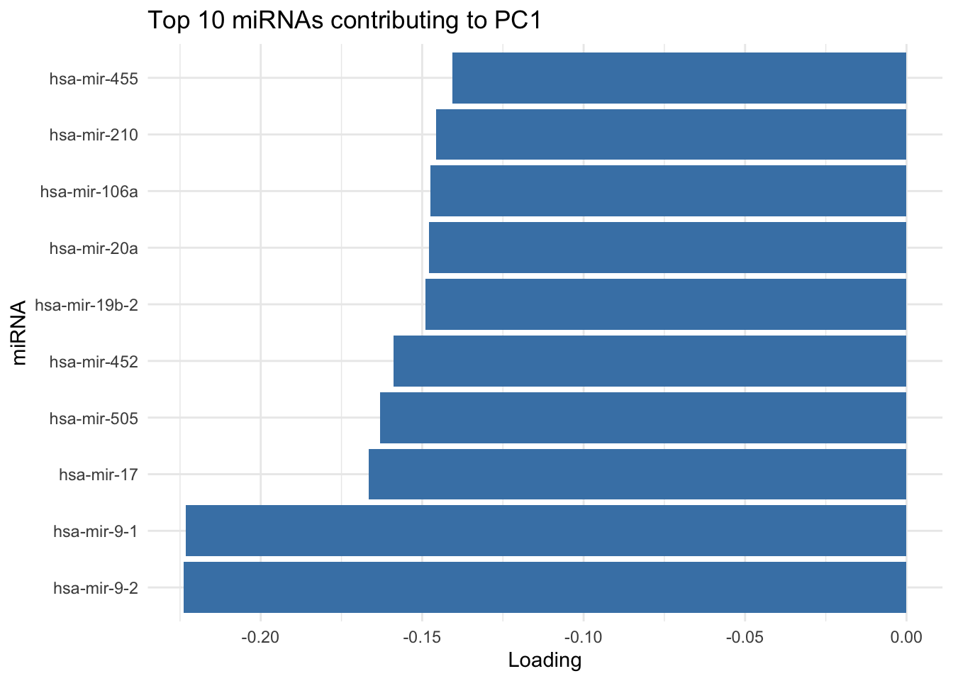

4.5 Run t-SNE

library(Rtsne)

x_scaled <- scale(x) # scale data

set.seed(42)
tsne_out <- Rtsne(x_scaled, dims = 2, perplexity = 30, verbose = TRUE)
## Performing PCA
## Read the 220 x 50 data matrix successfully!
## Using no_dims = 2, perplexity = 30.000000, and theta = 0.500000
## Computing input similarities...
## Building tree...
## Done in 0.02 seconds (sparsity = 0.563058)!
## Learning embedding...
## Iteration 50: error is 57.401944 (50 iterations in 0.02 seconds)
## Iteration 100: error is 55.085976 (50 iterations in 0.02 seconds)
## Iteration 150: error is 59.625533 (50 iterations in 0.02 seconds)
## Iteration 200: error is 58.073568 (50 iterations in 0.02 seconds)
## Iteration 250: error is 59.120896 (50 iterations in 0.03 seconds)
## Iteration 300: error is 1.614186 (50 iterations in 0.02 seconds)
## Iteration 350: error is 1.157171 (50 iterations in 0.02 seconds)
## Iteration 400: error is 0.940524 (50 iterations in 0.01 seconds)
## Iteration 450: error is 0.858315 (50 iterations in 0.01 seconds)
## Iteration 500: error is 0.822199 (50 iterations in 0.01 seconds)
## Iteration 550: error is 0.783186 (50 iterations in 0.02 seconds)
## Iteration 600: error is 0.777544 (50 iterations in 0.02 seconds)
## Iteration 650: error is 0.775445 (50 iterations in 0.02 seconds)
## Iteration 700: error is 0.775674 (50 iterations in 0.01 seconds)
## Iteration 750: error is 0.775880 (50 iterations in 0.02 seconds)
## Iteration 800: error is 0.776062 (50 iterations in 0.01 seconds)
## Iteration 850: error is 0.776889 (50 iterations in 0.01 seconds)
## Iteration 900: error is 0.776736 (50 iterations in 0.01 seconds)
## Iteration 950: error is 0.777065 (50 iterations in 0.01 seconds)
## Iteration 1000: error is 0.776988 (50 iterations in 0.01 seconds)
## Fitting performed in 0.34 seconds.

# Key parameters
# - perplexity: Balances local/global structure (recommended: 5–50)
# - dims: Output dimensions (2D or 3D)
# - theta: Speed/accuracy tradeoff
# - max_iter: Iteration count

tsne_df <- data.frame(
  X = tsne_out$Y[, 1],
  Y = tsne_out$Y[, 2],
  Subtype = labels
)

p_tsne <- ggplot(tsne_df, aes(x = X, y = Y, color = Subtype)) +
  geom_point(size = 2) +
  theme_minimal() +
  labs(title = "t-SNE on miRNA data") + 
  scale_color_manual(values = c("Basal" = "#FF0000", "Her2" = "#00FF00", "LumA" = "#0000FF"))

plot(p_tsne)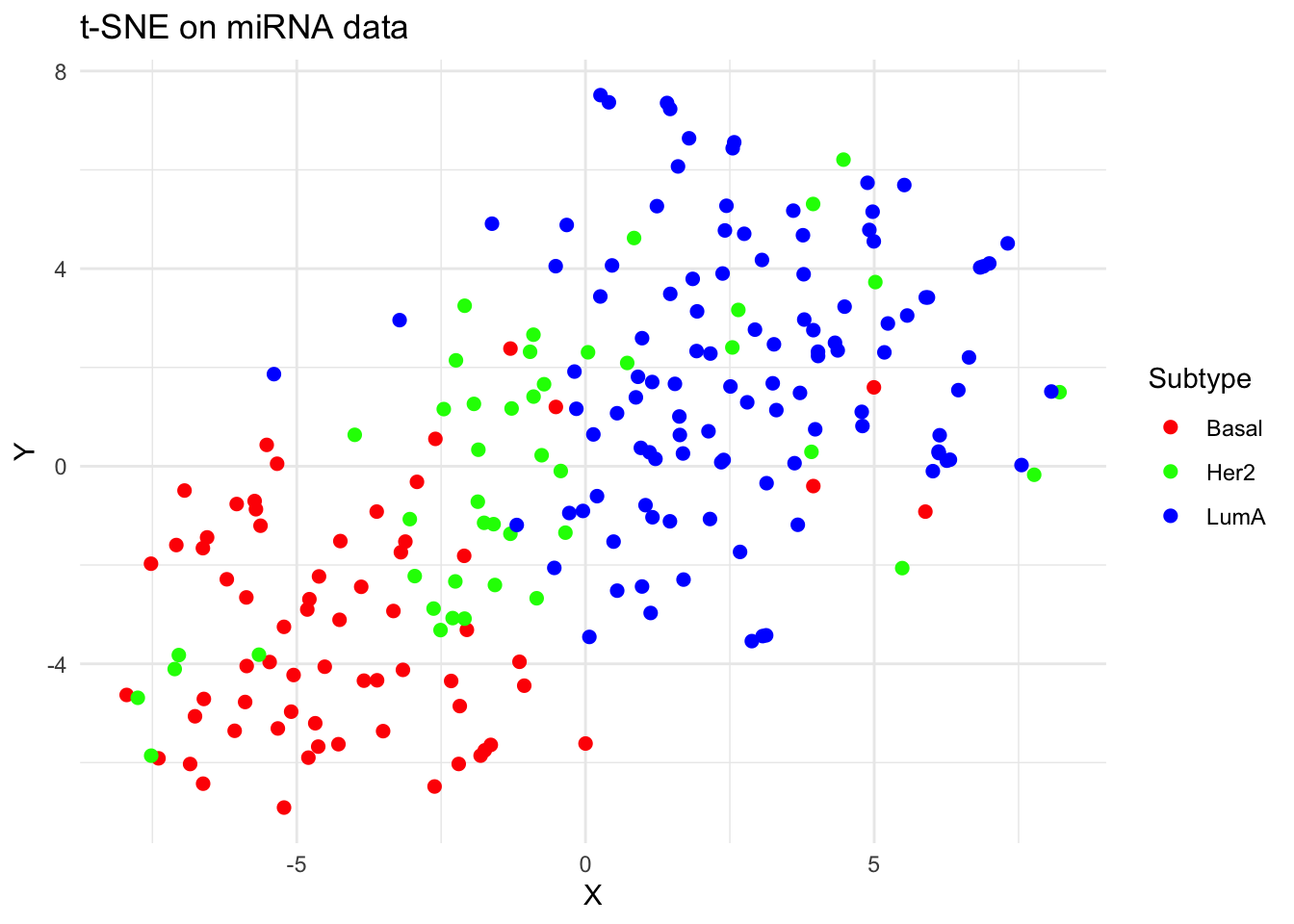

4.6 Run UMAP

library(umap)

set.seed(42)
umap_out <- umap(x_scaled)

# Key parameters
# - n_neighbors: Higher = more global structure
# - min_dist: Smaller = tighter clusters
# - metric: Distance measure (e.g., "euclidean")

umap_df <- data.frame(
  X = umap_out$layout[, 1],
  Y = umap_out$layout[, 2],
  Subtype = labels
)

p_umap <- ggplot(umap_df, aes(x = X, y = Y, color = Subtype)) +
  geom_point(size = 2) +
  theme_minimal() +
  labs(title = "UMAP on miRNA data") + 
  scale_color_manual(values = c("Basal" = "#FF0000", "Her2" = "#00FF00", "LumA" = "#0000FF"))

plot(p_umap)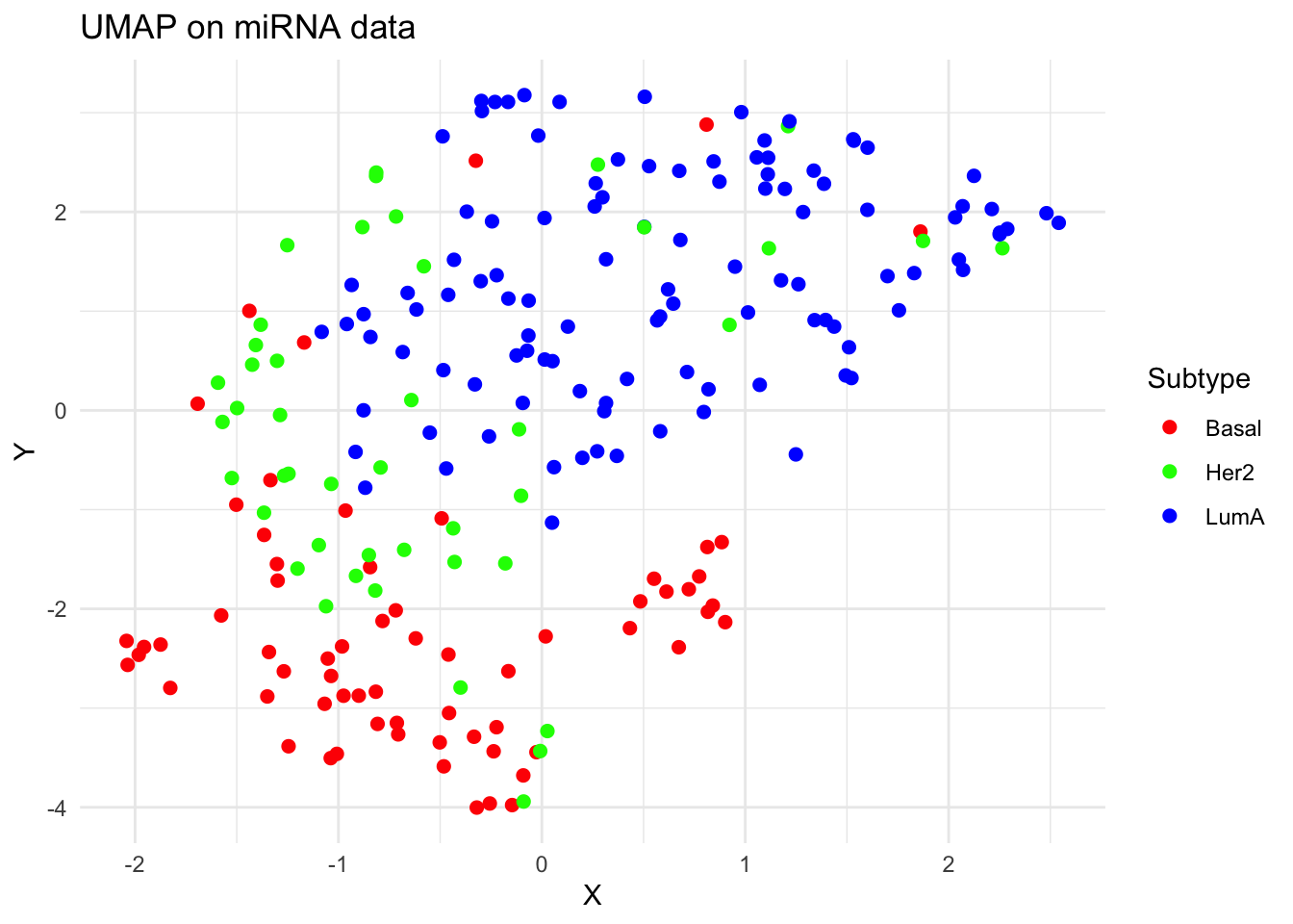

4.7 Compare PCA, t-SNE, and UMAP

library(patchwork)
p_pca + p_tsne + p_umap + plot_layout(ncol = 2)

4.8 Exercise (parameters exploration)

Try changing perplexity = 5, 50 in t-SNE. Try n_neighbors = 5, 30 in UMAP. Do you see different patterns? Why? Repeat the exercise with different random seed. Are t-SNE and UMAP sensitive to random initialization?

Example code

# t-SNE with perplexity = 10
set.seed(42)
tsne_5 <- Rtsne(x_scaled, dims = 2, perplexity = 5)
df_tsne5 <- data.frame(X = tsne_5$Y[,1], Y = tsne_5$Y[,2], Subtype = labels)

# t-SNE with perplexity = 50
set.seed(42)
tsne_50 <- Rtsne(x_scaled, dims = 2, perplexity = 50)
df_tsne50 <- data.frame(X = tsne_50$Y[,1], Y = tsne_50$Y[,2], Subtype = labels)

set.seed(42)
# UMAP with n_neighbors = 5
umap_5 <- umap(x_scaled, config = modifyList(umap.defaults, list(n_neighbors = 5)))
df_umap5 <- data.frame(X = umap_5$layout[,1], Y = umap_5$layout[,2], Subtype = labels)

set.seed(42)
# UMAP with n_neighbors = 30
umap_30 <- umap(x_scaled, config = modifyList(umap.defaults, list(n_neighbors = 30)))
df_umap30 <- data.frame(X = umap_30$layout[,1], Y = umap_30$layout[,2], Subtype = labels)

# Plot
library(patchwork)
p1 <- ggplot(df_tsne5, aes(X, Y, color = Subtype)) + geom_point() +
  ggtitle("t-SNE (perplexity = 5)") + theme_minimal()

p2 <- ggplot(df_tsne50, aes(X, Y, color = Subtype)) + geom_point() +
  ggtitle("t-SNE (perplexity = 50)") + theme_minimal()

p3 <- ggplot(df_umap5, aes(X, Y, color = Subtype)) + geom_point() +
  ggtitle("UMAP (n_neighbors = 5)") + theme_minimal()

p4 <- ggplot(df_umap30, aes(X, Y, color = Subtype)) + geom_point() +
  ggtitle("UMAP (n_neighbors = 30)") + theme_minimal()

p1 + p2 + p3 + p4

# Comments: 

# The comparison across parameter settings highlights how both t-SNE and UMAP balance local versus global structure depending on configuration:
# t-SNE (perplexity = 10):
# Shows very tight, localized groupings. Clusters are more fragmented, suggesting a strong focus on very close neighbors.
# t-SNE (perplexity = 50):
# Produces more continuous global structure. Classes are generally separated, but the fine local detail is smoothed out.
# UMAP (n_neighbors = 5):
# Strong emphasis on local clusters, resulting in a scattered, detailed structure with visible subgrouping. This may help detect subtypes or sub-clusters.
# UMAP (n_neighbors = 30):
# Prioritizes global structure. The major subtypes (Basal, Her2, LumA) appear as smoother, larger clusters, giving a clearer big-picture overview.

# Both t-SNE and UMAP are sensitive to the random seed because they rely on random initialization and stochastic optimization to construct the low-dimensional embedding. t-SNE is generally more sensitive because its cost function is non-convex and it places stronger emphasis on preserving local structure, making it more prone to variability in point arrangement across runs

4.9 Exercise (features variability)

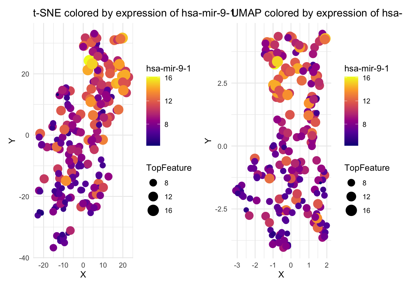
Investigate which miRNA features vary the most across the dataset. Features with high variance are more likely to influence clustering in dimensionality reduction. Identify top variable features in orginal (unscaled) data and visualize sample distribution colored by expression of top feature on the selected t-SNE and UMAP plots.