cd counts1 Learning outcomes
Using packages from Bioconductor:
to profile ATAC-seq signal by genomic location and by proximity to TSS regions;
to annotate peaks with the nearest feature;
to perform functional annotation.
Note
We continue working with data from (Tsao et al. 2022). We will use the count table derived from non subset data (already prepared).
We will also use results of Differential Accessibility.
Data processing recap: reads were mapped to reference genome mm39.
2 Introduction
In this tutorial we use an R / Bioconductor package ChIPseeker (Yu et al. 2015), to inspect the ATAC signal profiles (can be used for ChIP-seq as well), annotate peaks and visualise annotations. We will also perform functional annotation of peaks using clusterProfiler (Yu et al. 2012).
This tutorial is based on the ChIPseeker package tutorial so feel free to have this open alongside to read and experiment more.
3 Data & Methods
We will build upon the main labs:
ATAC-seq: all detected peaks (merged consensus peaks);
ATAC-seq: differentially accessible peaks;
4 Setting Up
You can continue working in the directory atacseq/analysis/counts. This directory contains merged peaks called earlier using genrich as well as count tables derived from summarising of non-subset data. Although strictly speaking we won’t need the count tables for this exercise, this will be our staring point, to prepare the object for the differential accessibility analysis. We will use file AB_Batf_KO_invivo.genrich_joint.merged_peaks.featureCounts and annotation libraries, which are preinstalled.
Note
We take advantage of the module system on Pelle in this tutorial. The code was tested under R 4.6.1 The lab was developed under the R version stated in session info.
We navigate to our working directory for this tutorial. Assuming we are at the top of the ataqseq/analysis
We access the R environment via:
module load R/4.6.1-gfbf-2026.1
module load R-bundle-CRAN/2026.07-foss-2026.1
module load R-bundle-Bioconductor/3.23-foss-2026.1-R-4.6.1
We activate R console upon typing R in the terminal.
To be able to load all necessary libraries we need to update the paths to custom library locations:
.libPaths(c(.libPaths(),"/proj/epi2026/library/Rpackages/4.6.1"))Alternatively you can work on this tutorial locally, using R libraries installed via renv.
We begin by loading necessary libraries:
library(tidyverse)
library(dplyr)
library(kableExtra)

library(GenomicRanges)

library(ChIPseeker)
library(ggupset)
library(ggimage)
library(biomaRt)
library(txdbmaker)
library(GenomicFeatures)

library(org.Mm.eg.db)
library(fgsea)
library(ReactomePA)
5 Preparing Annotations
We will use TSS and gene annotations from Ensembl. We can fetch them from biomaRt:
NoteObtaining the annotation objects
txdb_mm39 = txdbmaker::makeTxDbFromBiomart(biomart="ensembl",
                               dataset="mmusculus_gene_ensembl",
                               circ_seqs=NULL,
                               taxonomyId=NA)

ensembl = useEnsembl(biomart="genes", dataset="mmusculus_gene_ensembl")
all_genes = names(transcriptsBy(txdb_mm39, "gene"))

gene_annot_mm39=getBM(attributes =
   c('ensembl_gene_id', 'ensembl_transcript_id','external_gene_name','entrezgene_id','description','gene_biotype','chromosome_name','start_position','end_position','strand','transcription_start_site'),
       filters = 'ensembl_gene_id',
       values = all_genes,
        mart = ensembl)
We have prepared these annotation files for you, so you can load them via:
annotdir=file.path(getwd(),"annotation")

gene_annot_mm39=read.delim(file.path(annotdir,"mm39_gene_names.tab"), sep="\t", header=TRUE, quote = "")
and
pth_txdbens=file.path(annotdir,"Ensembl.txdb.GRCm39.Rdata")
txdb_mm39=loadDb(pth_txdbens)
You can inspect the objects:
txdb_mm39
## TxDb object:
## # Db type: TxDb
## # Supporting package: GenomicFeatures
## # Data source: BioMart
## # Organism: Mus musculus
## # Taxonomy ID: 10090
## # Resource URL: www.ensembl.org:443
## # BioMart database: ENSEMBL_MART_ENSEMBL
## # BioMart database version: Ensembl Genes 115
## # BioMart dataset: mmusculus_gene_ensembl
## # BioMart dataset description: Mouse genes (GRCm39)
## # BioMart dataset version: GRCm39
## # Full dataset: yes
## # miRBase build ID: NA
## # Nb of transcripts: 278396
## # Db created by: txdbmaker package from Bioconductor
## # Creation time: 2025-09-08 11:35:27 +0200 (Mon, 08 Sep 2025)
## # txdbmaker version at creation time: 1.0.1
## # RSQLite version at creation time: 2.4.3
## # DBSCHEMAVERSION: 1.2head(gene_annot_mm39)| ensembl_gene_id | ensembl_transcript_id | external_gene_name | entrezgene_id | description | gene_biotype | chromosome_name | start_position | end_position | strand | transcription_start_site |
|---|---|---|---|---|---|---|---|---|---|---|
| ENSMUSG00000000103 | ENSMUST00000187148 | Zfy2 | 22768 | zinc finger protein 2, Y-linked [Source:MGI Symbol;Acc:MGI:99213] | protein_coding | Y | 2106015 | 2170409 | -1 | 2150346 |
| ENSMUSG00000000103 | ENSMUST00000115891 | Zfy2 | 22768 | zinc finger protein 2, Y-linked [Source:MGI Symbol;Acc:MGI:99213] | protein_coding | Y | 2106015 | 2170409 | -1 | 2170409 |
| ENSMUSG00000001700 | ENSMUST00000237355 | Gramd2b | 107022 | GRAM domain containing 2B [Source:MGI Symbol;Acc:MGI:1914815] | protein_coding | 18 | 56533409 | 56636864 | 1 | 56533409 |
| ENSMUSG00000001700 | ENSMUST00000237422 | Gramd2b | 107022 | GRAM domain containing 2B [Source:MGI Symbol;Acc:MGI:1914815] | protein_coding | 18 | 56533409 | 56636864 | 1 | 56533447 |
| ENSMUSG00000001700 | ENSMUST00000235794 | Gramd2b | 107022 | GRAM domain containing 2B [Source:MGI Symbol;Acc:MGI:1914815] | protein_coding | 18 | 56533409 | 56636864 | 1 | 56552242 |
| ENSMUSG00000001700 | ENSMUST00000237716 | Gramd2b | 107022 | GRAM domain containing 2B [Source:MGI Symbol;Acc:MGI:1914815] | protein_coding | 18 | 56533409 | 56636864 | 1 | 56602339 |
NoteWorking with UCSC annotations
If you would rather annotate TSS using the gene models from UCSC you can use the Bioconductor package directly:
library(TxDb.Mmusculus.UCSC.mm39.knownGene)
txdb = TxDb.Hsapiens.UCSC.mm39.knownGene
Please note that UCSC and Ensembl use different contig naming schemes, so it is advisable to use the annotation matching the genome reference used for read mapping.
6 Data
We can now load data:
count_table_fname="AB_Batf_KO_invivo.genrich_joint.merged_peaks.featureCounts"
cnt_table=read.table(count_table_fname, sep="\t", header=TRUE, blank.lines.skip=TRUE)
We will format the column names and subset the count table to only contain the peaks on assembled chromosomes.
rownames(cnt_table)=cnt_table$Geneid
rownames(cnt_table)=c(gsub("AB_Batf_KO_invivo.genrich_joint.","",rownames(cnt_table)))
colnames(cnt_table)=c(colnames(cnt_table)[1:6],gsub(".filt.bam","",colnames(cnt_table)[7:10]))

colnames(cnt_table)[7:10]=c("B1_WT_Batf-floxed","B2_WT_Batf-floxed","A1_Batf_cKO","A2_Batf_cKO")

#remove peaks not on the assembled chromosomes
cnt_table_chr=cnt_table|>
  dplyr::filter(Chr%in%c(1:19) | Chr%in%c("X","Y"))

reads.peak=cnt_table_chr[,c(7:10)]

head(reads.peak)| B1_WT_Batf-floxed | B2_WT_Batf-floxed | A1_Batf_cKO | A2_Batf_cKO | |
|---|---|---|---|---|
| merged_peaks_1 | 299 | 238 | 325 | 330 |
| merged_peaks_2 | 106 | 83 | 162 | 174 |
| merged_peaks_3 | 19 | 24 | 25 | 21 |
| merged_peaks_4 | 27 | 31 | 40 | 29 |
| merged_peaks_5 | 114 | 101 | 65 | 151 |
| merged_peaks_6 | 129 | 137 | 120 | 204 |
All peaks: n = 65027;
Peaks on assembled chromosomes: n = 64879. These peaks will be used for further analysis.
7 Peak Annotation
We will be working on a GRanges object peaks_gr containing non-subset peaks (i.e. all assebled chromosome peaks).
We create the GRanges object:
peaks_gr=GRanges(seqnames=cnt_table_chr$Chr, ranges=IRanges(cnt_table_chr$Start, cnt_table_chr$End), strand="*", mcols=data.frame(peakID=rownames(cnt_table_chr)))and inspect it:
peaks_gr
## GRanges object with 64879 ranges and 1 metadata column:
##           seqnames            ranges strand |       mcols.peakID
##              <Rle>         <IRanges>  <Rle> |        <character>
##       [1]        1   3050939-3052959      * |     merged_peaks_1
##       [2]        1   3053048-3054634      * |     merged_peaks_2
##       [3]        1   3054861-3055532      * |     merged_peaks_3
##       [4]        1   3057260-3057785      * |     merged_peaks_4
##       [5]        1   3059375-3061360      * |     merged_peaks_5
##       ...      ...               ...    ... .                ...
##   [64875]        Y 90814281-90815165      * | merged_peaks_64875
##   [64876]        Y 90815739-90816707      * | merged_peaks_64876
##   [64877]        Y 90818033-90819321      * | merged_peaks_64877
##   [64878]        Y 90819900-90820364      * | merged_peaks_64878
##   [64879]        Y 90821996-90824312      * | merged_peaks_64879
##   -------
##   seqinfo: 21 sequences from an unspecified genome; no seqlengths
We are ready to annotate the peaks to their closest feature:
peakAnno=annotatePeak(peaks_gr, tssRegion=c(-3000, 3000),TxDb=txdb_mm39)Summary of the regions annotated to peaks:
peakAnno
## Annotated peaks generated by ChIPseeker
## 64879/64879  peaks were annotated
## Genomic Annotation Summary:
##               Feature   Frequency
## 9    Promoter (<=1kb) 36.09642565
## 10   Promoter (1-2kb)  8.69464696
## 11   Promoter (2-3kb)  6.88204196
## 4              5' UTR  0.12022380
## 3              3' UTR  1.63843462
## 1            1st Exon  0.04469859
## 7          Other Exon  3.04104564
## 2          1st Intron 10.21594044
## 8        Other Intron 18.13838068
## 6  Downstream (<=300)  0.13717844
## 5   Distal Intergenic 14.99098321
Over 30% peaks localised to TSS, as expected in an ATAC-seq experiment.
To inspect peak annotations:
peakAnno_df=as.data.frame(peakAnno)head(peakAnno_df)| seqnames | start | end | width | strand | mcols.peakID | annotation | geneChr | geneStart | geneEnd | geneLength | geneStrand | geneId | transcriptId | distanceToTSS |
|---|---|---|---|---|---|---|---|---|---|---|---|---|---|---|
| 1 | 3050939 | 3052959 | 2021 | * | merged_peaks_1 | Distal Intergenic | 1 | 3143476 | 3144545 | 1070 | 1 | ENSMUSG00000102693 | ENSMUST00000193812 | -90517 |
| 1 | 3053048 | 3054634 | 1587 | * | merged_peaks_2 | Distal Intergenic | 1 | 3143476 | 3144545 | 1070 | 1 | ENSMUSG00000102693 | ENSMUST00000193812 | -88842 |
| 1 | 3054861 | 3055532 | 672 | * | merged_peaks_3 | Distal Intergenic | 1 | 3143476 | 3144545 | 1070 | 1 | ENSMUSG00000102693 | ENSMUST00000193812 | -87944 |
| 1 | 3057260 | 3057785 | 526 | * | merged_peaks_4 | Distal Intergenic | 1 | 3143476 | 3144545 | 1070 | 1 | ENSMUSG00000102693 | ENSMUST00000193812 | -85691 |
| 1 | 3059375 | 3061360 | 1986 | * | merged_peaks_5 | Distal Intergenic | 1 | 3143476 | 3144545 | 1070 | 1 | ENSMUSG00000102693 | ENSMUST00000193812 | -82116 |
| 1 | 3066555 | 3069092 | 2538 | * | merged_peaks_6 | Distal Intergenic | 1 | 3143476 | 3144545 | 1070 | 1 | ENSMUSG00000102693 | ENSMUST00000193812 | -74384 |
We may want to include more gene related information:
peakAnno_df=peakAnno_df|>
  left_join(gene_annot_mm39, by=c("transcriptId"="ensembl_transcript_id"))|>
  dplyr::rename(peakID=mcols.peakID)
NoteAnnotated peaks can be saved to a file as a table or rds object
write.table(peakAnno_df, "Batf_WT_KO.merged_peaks.tsv",
    append = FALSE,
    quote = FALSE,
    sep = "\t",
    row.names = FALSE,
    col.names = TRUE,
    fileEncoding = "")
We can also assess the read density at annotated TSS regions. The plot of read density at the transcription start sites (TSS) for all peaks is presented on Figure 1.
promoter=getPromoters(TxDb=txdb_mm39, upstream=3000, downstream=3000)tagMatrix=getTagMatrix(peaks_gr, windows=promoter)
## >> preparing start_site regions by gene... 2026-10-09 13:45:57
## >> preparing tag matrix... 2026-10-09 13:45:57
TSS_profile=plotAvgProf(tagMatrix, xlim=c(-3000, 3000), xlab="Genomic Region (5'->3')", ylab = "Read Count in Peaks")
## >> plotting figure... 2026-10-09 13:46:25TSS_profile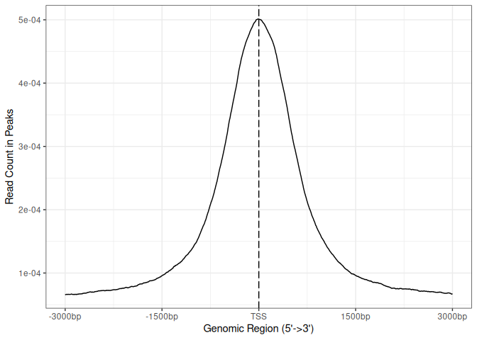
We can also plot summary of the annotations:
peakAnnoplot=upsetplot(peakAnno, vennpie=TRUE)peakAnnoplot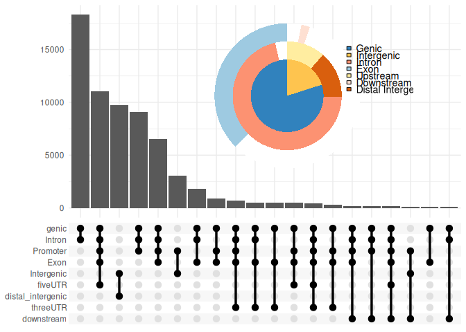
NoteSaving the plots
pdf("TSSdist.pdf")
  TSS_profile
dev.off()

pdf("AnnotVis.pdf")
  peakAnnoplot
dev.off()
8 Functional Analysis
Having obtained annotations to nearest genes, we can perform functional enrichment analysis to identify predominant biological themes among these genes by incorporating knowledge provided by biological ontologies, e.g. GO (Gene Ontology, (Ashburner et al. 2000)) and Reactome (Griss et al. 2020).
We can use several approaches and peak sets for this, e.g.:
genes annotated to merged consensus peaks set in e.g. promoters or proximal to TSS to assess functional signature in open chromatin regions (OCRs) (overrepresentation analysis set vs. id universe, ORA);
differentially accessible peaks to define functional signature in OCRs which change their occupancy status (ORA);
genes annotated to merged consensus peaks set ranked by an effect size metric (Gene Set Enrichment Analysis, GSEA).
8.1 Pathway Over-Representation Analysis
Overrepresentation analysis (ORA) is a method to test whether genes within given gene set are overepresented in the subset (open chromatin, DA peaks, etc.) vs. the universe (all genes).
Let’s first annotate the consensus peaks, representing open chromatin regions (OCRs) with Reactome pathways.
Reactome uses entrez gene ID space for gene - pathway annotation.
Reactome pathway enrichment of genes defined as the nearest feature to the peaks:
entrez_ids=peakAnno_df$entrezgene_id
entrez_ids=entrez_ids[!is.na(unique(entrez_ids))]

pathway.reac=ReactomePA::enrichPathway(entrez_ids, organism = "mouse")
#previewing enriched Reactome pathways
colnames(as.data.frame(pathway.reac))
##  [1] "ID"             "Description"    "GeneRatio"      "BgRatio"
##  [5] "RichFactor"     "FoldEnrichment" "zScore"         "pvalue"
##  [9] "p.adjust"       "qvalue"         "geneID"         "Count"

#we skip the preview of some columns which contain long strings of gene IDs
pathway.reac[1:10,c(1:7,9)]| ID | Description | GeneRatio | BgRatio | RichFactor | FoldEnrichment | zScore | p.adjust | |
|---|---|---|---|---|---|---|---|---|
| R-MMU-983168 | R-MMU-983168 | Antigen processing: Ubiquitination & Proteasome degradation | 259/6844 | 274/8851 | 0.9452555 | 1.222451 | 6.907094 | 0.0e+00 |
| R-MMU-983169 | R-MMU-983169 | Class I MHC mediated antigen processing & presentation | 301/6844 | 326/8851 | 0.9233129 | 1.194074 | 6.592982 | 0.0e+00 |
| R-MMU-9012999 | R-MMU-9012999 | RHO GTPase cycle | 355/6844 | 390/8851 | 0.9102564 | 1.177189 | 6.608615 | 0.0e+00 |
| R-MMU-2555396 | R-MMU-2555396 | Mitotic Metaphase and Anaphase | 192/6844 | 207/8851 | 0.9275362 | 1.199536 | 5.364159 | 4.0e-07 |
| R-MMU-1280215 | R-MMU-1280215 | Cytokine Signaling in Immune system | 397/6844 | 451/8851 | 0.8802661 | 1.138404 | 5.571207 | 4.0e-07 |
| R-MMU-68882 | R-MMU-68882 | Mitotic Anaphase | 191/6844 | 206/8851 | 0.9271845 | 1.199081 | 5.338677 | 4.0e-07 |
| R-MMU-3700989 | R-MMU-3700989 | Transcriptional Regulation by TP53 | 252/6844 | 279/8851 | 0.9032258 | 1.168096 | 5.268322 | 1.3e-06 |
| R-MMU-8951664 | R-MMU-8951664 | Neddylation | 188/6844 | 204/8851 | 0.9215686 | 1.191818 | 5.118293 | 1.8e-06 |
| R-MMU-73887 | R-MMU-73887 | Death Receptor Signaling | 130/6844 | 137/8851 | 0.9489051 | 1.227171 | 4.948318 | 1.9e-06 |
| R-MMU-69620 | R-MMU-69620 | Cell Cycle Checkpoints | 247/6844 | 275/8851 | 0.8981818 | 1.161573 | 5.026276 | 4.8e-06 |
We can see familar terms which can be connected to sample biology:
Cytokine Signaling in Immune system
Class I MHC mediated antigen processing & presentation
8.2 Gene Set Enrichment Analysis
Gene set enrichment analysis (GSEA) is a test whether gene set member genes are present towards to top of the ranked list of genes (Subramanian et al. 2005). The rank usually corresponds to the effect size and statistical significance. Ties in the ranked list are discouraged, as they may lead to unexpected results.
We can check for GO terms enriched amongst DA OCRs by using GSEA.
We need to read in the results of the DA analysis:
DA_res=readRDS("../../results/DA/objects/Batf_WT_KO.merged_peaks.DA_TMM.annot.rds")The metric to use in GSEA ideally should combine effect size and statistical significance.
Common practice for constructing the metric based on edgeR results is:
DA_res=DA_res|>
  dplyr::mutate(gsea_metric=PValue*logFC)
GSEA statistical framework recommends that the ranked gene list is duplicate free; yet often a gene may have more than one peak annotated. If we leave the list as is (i.e. with duplicated gene ids and different value for ranking metric for each entry), we have no control over which peak / metric value gets selected for GSEA, which may lead to unexpected results. Applying some selection strategy for genes with multiple peaks helps with interpretability of the GSEA results.
In this tutorial, we select:
genes with ATAC peaks up to 3 kb of their TSS (annotated as
Promoter);one peak per gene; we select the peak with largest absolute fold change;
This will require some data wrangling:
DA_res.prom.top=DA_res|>
  dplyr::mutate(gene_name=coalesce(external_gene_name,geneId))|>
  dplyr::filter(annotation%in%c("Promoter"))|>
  dplyr::group_by(gene_name)|>
  dplyr::mutate(gene_max_abs_lfc=max(abs(logFC)))|>
  dplyr::ungroup()|>
  dplyr::rowwise()|>
  dplyr::filter(abs(logFC)==gene_max_abs_lfc)|>
  dplyr::distinct(gene_name, .keep_all=TRUE)|>
  as.data.frame()

## we also need to add entrez gene id and clean up entries without it
DA_res.prom.top=DA_res.prom.top|>
    left_join(gene_annot_mm39[,c(2,4)], by=c("transcriptId"="ensembl_transcript_id"))|>
    dplyr::distinct(entrezgene_id, .keep_all=TRUE)|>
    dplyr::filter_at(vars(entrezgene_id), all_vars(!is.na(.)))
We can now create a named list (names are entrez gene id) and sort it:
gene_list=DA_res.prom.top$gsea_metric #using pval*logFC
names(gene_list)=DA_res.prom.top$entrezgene_id
gene_list=gene_list[order(gene_list,decreasing=TRUE)]

head(gene_list)
We prepare the GO terms and run GSEA:
all_go.bp=as.data.frame(org.Mm.egGO)|>
  dplyr::filter(Ontology=="BP")

go_terms=as.list(org.Mm.egGO2ALLEGS)
go_terms=go_terms[names(go_terms)%in%all_go.bp$go_id]

gsea_go=fgsea(pathways = go_terms,
                  stats    = gene_list,
                  minSize  = 15,
                  maxSize  = 500,
                  scoreType    = "std")
The resulting object contains basic statistics of the GSEA test.
 head(gsea_go)
     pathway      pval      padj    log2err         ES        NES size
1 GO:0000018 0.9928571 1.0000000 0.05400883  0.1824006  0.6768697  120
2 GO:0000027 0.9490446 1.0000000 0.05080541  0.2415674  0.6675675   24
3 GO:0000028 0.1902072 0.8391112 0.13649044 -0.4844570 -1.2474683   19
4 GO:0000038 0.2611111 0.8800840 0.11284336 -0.4165674 -1.1610107   27
5 GO:0000041 0.3404255 0.9065779 0.09374654 -0.2997705 -1.0499786   83
6 GO:0000045 0.3294118 0.8975844 0.11331291  0.2753809  1.0549553  137
   leadingEdge
1 19264, 7....
2 72831, 2....
3 67097, 9....
4 14081, 1....
5 226025, ....
6 240327, ....
We can format these results:
gsea_go=as.data.frame(gsea_go)

library(GO.db)
go_terms=select(GO.db, columns=c("GOID","TERM"), keys=gsea_go$pathway, keytype="GOID")

gsea_go=gsea_go|>
    dplyr::filter(pval<0.01)|>
    dplyr::select(pathway,NES,pval,padj,size)|>
    left_join(go_terms, by=c("pathway"="GOID"))

> head(gsea_go)
     pathway       NES        pval      padj size                         TERM
1 GO:0002064 -1.539558 0.001013134 0.5754347  181  epithelial cell development
2 GO:0003014 -1.542754 0.004758923 0.5757116   85         renal system process
3 GO:0006814 -1.434938 0.006011068 0.5757116  171         sodium ion transport
4 GO:0006836 -1.473969 0.002957773 0.5754347  184   neurotransmitter transport
5 GO:0007431 -1.702995 0.003805549 0.5757116   31   salivary gland development
6 GO:0007435 -1.738422 0.002137247 0.5754347   27 salivary gland morphogenesis
Upon object inspection we can see terms related to immune cell biology, amongst other GO terms.
antigen processing and presentation (GO:0019882)
antigen processing and presentation of peptide antigen (GO:0048002)
9 Session Info
NoteSession Info
sessionInfo()
## R version 4.6.1 (2026-06-24)
## Platform: x86_64-pc-linux-gnu
## Running under: Ubuntu 24.04.5 LTS
##
## Matrix products: default
## BLAS:   /usr/lib/x86_64-linux-gnu/openblas-pthread/libblas.so.3
## LAPACK: /usr/lib/x86_64-linux-gnu/openblas-pthread/libopenblasp-r0.3.26.so;  LAPACK version 3.12.0
##
## locale:
##  [1] LC_CTYPE=C.UTF-8       LC_NUMERIC=C           LC_TIME=C.UTF-8
##  [4] LC_COLLATE=C.UTF-8     LC_MONETARY=C.UTF-8    LC_MESSAGES=C.UTF-8
##  [7] LC_PAPER=C.UTF-8       LC_NAME=C              LC_ADDRESS=C
## [10] LC_TELEPHONE=C         LC_MEASUREMENT=C.UTF-8 LC_IDENTIFICATION=C
##
## time zone: UTC
## tzcode source: system (glibc)
##
## attached base packages:
## [1] stats4    stats     graphics  grDevices datasets  utils     methods
## [8] base
##
## other attached packages:
##  [1] ReactomePA_1.56.0      fgsea_1.38.0           org.Mm.eg.db_3.23.0
##  [4] txdbmaker_1.8.0        GenomicFeatures_1.64.0 AnnotationDbi_1.74.0
##  [7] Biobase_2.72.0         biomaRt_2.68.0         ggimage_0.3.5
## [10] ggupset_0.4.1          ChIPseeker_1.48.0      GenomicRanges_1.64.0
## [13] Seqinfo_1.2.0          IRanges_2.46.0         S4Vectors_0.50.2
## [16] BiocGenerics_0.58.1    generics_0.1.4         kableExtra_1.4.1
## [19] lubridate_1.9.5        forcats_1.0.1          stringr_1.6.0
## [22] dplyr_1.2.1            purrr_1.2.2            readr_2.2.0
## [25] tidyr_1.3.2            tibble_3.3.1           ggplot2_4.0.3
## [28] tidyverse_2.0.0        knitr_1.51
##
## loaded via a namespace (and not attached):
##   [1] splines_4.6.1
##   [2] BiocIO_1.22.0
##   [3] bitops_1.0-9
##   [4] ggplotify_0.1.3
##   [5] filelock_1.0.3
##   [6] polyclip_1.10-7
##   [7] graph_1.90.0
##   [8] enrichit_0.2.4
##   [9] XML_3.99-0.23
##  [10] lifecycle_1.0.5
##  [11] httr2_1.2.2
##  [12] lattice_0.22-9
##  [13] MASS_7.3-65
##  [14] magrittr_2.0.5
##  [15] rmarkdown_2.31
##  [16] yaml_2.3.12
##  [17] plotrix_3.8-14
##  [18] otel_0.2.0
##  [19] ggtangle_0.1.2
##  [20] cowplot_1.2.0
##  [21] DBI_1.3.0
##  [22] RColorBrewer_1.1-3
##  [23] abind_1.4-8
##  [24] ggraph_2.2.2
##  [25] RCurl_1.98-1.18
##  [26] yulab.utils_0.2.5
##  [27] tweenr_2.0.3
##  [28] rappdirs_0.3.4
##  [29] gdtools_0.5.1
##  [30] enrichplot_1.32.0
##  [31] ggrepel_0.9.8
##  [32] tidytree_0.4.8
##  [33] reactome.db_1.96.0
##  [34] svglite_2.2.2
##  [35] codetools_0.2-20
##  [36] DelayedArray_0.38.1
##  [37] DOSE_4.6.0
##  [38] xml2_1.6.0
##  [39] ggforce_0.5.0
##  [40] tidyselect_1.2.1
##  [41] aplot_0.3.1
##  [42] UCSC.utils_1.8.0
##  [43] farver_2.1.2
##  [44] viridis_0.6.5
##  [45] matrixStats_1.5.0
##  [46] BiocFileCache_3.2.0
##  [47] GenomicAlignments_1.48.0
##  [48] jsonlite_2.0.0
##  [49] tidygraph_1.3.1
##  [50] systemfonts_1.3.2
##  [51] tools_4.6.1
##  [52] ggnewscale_0.5.2
##  [53] progress_1.2.3
##  [54] treeio_1.36.1
##  [55] TxDb.Hsapiens.UCSC.hg19.knownGene_3.22.1
##  [56] Rcpp_1.1.1-1.1
##  [57] glue_1.8.1
##  [58] gridExtra_2.3.1
##  [59] SparseArray_1.12.2
##  [60] xfun_0.57
##  [61] qvalue_2.44.0
##  [62] MatrixGenerics_1.24.0
##  [63] GenomeInfoDb_1.48.0
##  [64] withr_3.0.2
##  [65] BiocManager_1.30.27
##  [66] fastmap_1.2.0
##  [67] boot_1.3-32
##  [68] caTools_1.18.3
##  [69] digest_0.6.39
##  [70] timechange_0.4.0
##  [71] R6_2.6.1
##  [72] gridGraphics_0.5-1
##  [73] textshaping_1.0.5
##  [74] GO.db_3.23.1
##  [75] gtools_3.9.5
##  [76] dichromat_2.0-1
##  [77] RSQLite_3.53.1
##  [78] cigarillo_1.2.0
##  [79] data.table_1.18.6.1
##  [80] fontLiberation_0.1.0
##  [81] renv_1.2.3
##  [82] rtracklayer_1.72.0
##  [83] graphlayouts_1.2.5
##  [84] prettyunits_1.2.0
##  [85] httr_1.4.8
##  [86] htmlwidgets_1.6.4
##  [87] S4Arrays_1.12.1
##  [88] scatterpie_0.2.6
##  [89] graphite_1.58.0
##  [90] pkgconfig_2.0.3
##  [91] gtable_0.3.6
##  [92] blob_1.3.0
##  [93] S7_0.2.2
##  [94] XVector_0.52.0
##  [95] htmltools_0.5.9
##  [96] fontBitstreamVera_0.1.1
##  [97] scales_1.4.0
##  [98] png_0.1-9
##  [99] ggfun_0.2.1
## [100] rstudioapi_0.19.0
## [101] tzdb_0.5.0
## [102] reshape2_1.4.5
## [103] rjson_0.2.23
## [104] nlme_3.1-169
## [105] curl_7.1.0
## [106] cachem_1.1.0
## [107] KernSmooth_2.23-26
## [108] parallel_4.6.1
## [109] restfulr_0.0.16
## [110] pillar_1.11.1
## [111] grid_4.6.1
## [112] vctrs_0.7.3
## [113] gplots_3.3.0
## [114] tidydr_0.0.6
## [115] dbplyr_2.5.2
## [116] cluster_2.1.8.2
## [117] evaluate_1.0.5
## [118] magick_2.9.1
## [119] cli_3.6.6
## [120] compiler_4.6.1
## [121] Rsamtools_2.28.0
## [122] rlang_1.3.0
## [123] crayon_1.5.3
## [124] labeling_0.4.3
## [125] plyr_1.8.9
## [126] fs_2.1.0
## [127] ggiraph_0.9.6
## [128] stringi_1.8.7
## [129] viridisLite_0.4.3
## [130] BiocParallel_1.46.0
## [131] Biostrings_2.80.0
## [132] lazyeval_0.2.3
## [133] GOSemSim_2.38.3
## [134] fontquiver_0.2.1
## [135] Matrix_1.7-5
## [136] hms_1.1.4
## [137] patchwork_1.3.2
## [138] bit64_4.8.2
## [139] KEGGREST_1.52.0
## [140] SummarizedExperiment_1.42.0
## [141] igraph_2.3.3
## [142] memoise_2.0.1
## [143] ggtree_4.2.0
## [144] fastmatch_1.1-8
## [145] bit_4.6.0
## [146] gson_0.2.1
## [147] ape_5.8-1
10 References
Ashburner, M., C. A. Ball, J. A. Blake, et al. 2000. “Gene ontology: tool for the unification of biology. The Gene Ontology Consortium.” Nat Genet 25 (1): 25–29.
Griss, J., G. Viteri, K. Sidiropoulos, V. Nguyen, A. Fabregat, and H. Hermjakob. 2020. “ReactomeGSA - Efficient Multi-Omics Comparative Pathway Analysis.” Mol Cell Proteomics 19 (12): 2115–25.
Subramanian, A., P. Tamayo, V. K. Mootha, et al. 2005. “Gene set enrichment analysis: a knowledge-based approach for interpreting genome-wide expression profiles.” Proc Natl Acad Sci U S A 102 (43): 15545–50.
Tsao, Hsiao-Wei, James Kaminski, Makoto Kurachi, et al. 2022. “Batf-Mediated Epigenetic Control of Effector CD8 + t Cell Differentiation.” Science Immunology 7 (68). https://doi.org/10.1126/sciimmunol.abi4919.
Yu, Guangchuang, Li-Gen Wang, Yanyan Han, and Qing-Yu He. 2012. “clusterProfiler: An r Package for Comparing Biological Themes Among Gene Clusters.” OMICS: A Journal of Integrative Biology 16 (5): 284–87. https://doi.org/10.1089/omi.2011.0118.
Yu, Guangchuang, Li-Gen Wang, and Qing-Yu He. 2015. “ChIPseeker: An r/Bioconductor Package for ChIP Peak Annotation, Comparison and Visualization.” Bioinformatics 31 (14): 2382–83. https://doi.org/10.1093/bioinformatics/btv145.