ATAC-seq Peak Differential Accessibility

1 Learning outcomes

Using packages from Bioconductor:

• to assess GC bias in ATAC-seq data;

• to select appropriate scaling normalisation of ATAC-seq data;

• to detect differentially accessible regions using edgeR.

Note

We continue working with data from (Tsao et al. 2022). We will use the count table derived from non subset data (already prepared).

Optionally, we will also use peaks annotated to closest genomic feature obtained as described in Peak Annotation.

Data processing recap: reads were mapped to reference genome mm39.

2 Introduction

In this tutorial we use an R / Bioconductor packages edgeR (Robinson and Oshlack 2010), (Chen et al. 2016), EDASeq (Risso et al. 2011) and cqn (Hansen et al. 2012) to perform normalisation and analysis of differential accessibility in ATAC-seq data.

3 Data & Methods

We will build upon the main lab ATACseq data analysis:

• we will interrogate GC bias in peaks and in adjacent non-overlapping genomic bins;

• we will use the counts table encompassing complete data for differential accessibility analysis;

3.1 Setting Up

You can continue working in the directory atacseq/analysis/counts. This directory contains merged peaks called earlier using Genrich as well as count tables derived from summarising of non-subset data. We will use file AB_Batf_KO_invivo.genrich_joint.merged_peaks.featureCounts.

Note

We take advantage of the module system on Pelle in this tutorial. The code was tested under R 4.6.1 The lab was developed under the R version stated in session info.

We access the R environment via:

module load R_packages/4.6.1

We activate R console upon typing R in the terminal.

We begin by loading necessary libraries:

library(tidyverse)
library(dplyr)
library(kableExtra)

library(ggplot2)
library(wesanderson)

library(GenomicRanges)
library(Hmisc)
library(Biostrings)
library(regioneR)
require(MASS)

library(BSgenome.Mmusculus.UCSC.mm39)

library(edgeR)
library(limma)
library(SummarizedExperiment)
library(EDASeq)
library(cqn)

4 Data

We can now load data. We will subset the count table to only contain the peaks on assembled chromosomes.

count_table_fname="AB_Batf_KO_invivo.genrich_joint.merged_peaks.featureCounts"
#cnt_table_pth=file.path(file.path(workdir,"assets","data"),count_table_fname)


cnt_table_pth=file.path(file.path("assets","data"),count_table_fname)


cnt_table=read.table(cnt_table_pth, sep="\t", header=TRUE, blank.lines.skip=TRUE)
rownames(cnt_table)=cnt_table$Geneid
rownames(cnt_table)=c(gsub("AB_Batf_KO_invivo.genrich_joint.","",rownames(cnt_table)))
colnames(cnt_table)=c(colnames(cnt_table)[1:6],gsub(".filt.bam","",colnames(cnt_table)[7:10]))

colnames(cnt_table)[7:10]=c("B1_WT_Batf-floxed","B2_WT_Batf-floxed","A1_Batf_cKO","A2_Batf_cKO")

#remove peaks not on the assembled chromosomes
cnt_table_chr=cnt_table|>
  dplyr::filter(Chr%in%c(1:19) | Chr%in%c("X","Y"))

reads.peak=cnt_table_chr[,c(7:10)]

head(reads.peak)

	B1_WT_Batf-floxed	B2_WT_Batf-floxed	A1_Batf_cKO	A2_Batf_cKO
merged_peaks_1	299	238	325	330
merged_peaks_2	106	83	162	174
merged_peaks_3	19	24	25	21
merged_peaks_4	27	31	40	29
merged_peaks_5	114	101	65	151
merged_peaks_6	129	137	120	204

• All peaks: n = 65027;

• Peaks on assembled chromosomes: n = 64879. These peaks will be used for further analysis.

5 GC Bias

5.1 GC Bias in Genomic Bins

To ivestigate the GC bias in adjacent genomic bins (background), we start with creating the GRanges object holding the tiled genome intervals. We will do it for one chromosome only (chr1), to save compute time.

chr.lengths = seqlengths(Mmusculus)[1:21]
chr.lengths.chr1=chr.lengths[1]

#tiles
tiles_chr1=GenomicRanges::tileGenome(chr.lengths.chr1,tilewidth=5000, cut.last.tile.in.chrom=TRUE)

#sequence
tileSeqs=BSgenome::getSeq(Mmusculus,tiles_chr1)

#GCcontent
gcContentTiles=Biostrings::letterFrequency(tileSeqs, "GC",as.prob=TRUE)[,1]
mcols(tiles_chr1)$gc=gcContentTiles

We need to tweak chromosome names to match the genome reference used for read mapping:

# tiles_chr1
# remove chr from granges obj
seqlevels(tiles_chr1)=gsub("chr","",seqlevels(tiles_chr1))

We can now count reads in all bam files in the data set, and plot them.

# comment this out for production on gh-pages
bam_dir="/Users/agatasmialowska/NBIS/fr_backup/teaching/epigenomics/labs2025/atacseq/Tsao2022/bam"

bam_fnames=list.files(bam_dir,pattern = "\\.bam$",)

bam_cnts_bins=list()

for (bam_fname in bam_fnames){

    bam_path=file.path(bam_dir,bam_fname)

    tiles_bam=tiles_chr1

    tiled_counts=bamCount(bam_path, tiles_bam, verbose=FALSE)
    mcols(tiles_bam)$readcount=tiled_counts

    bam_cnts_bins[[bam_fname]]=tiles_bam

}

saveRDS(bam_cnts_bins, 
  file = "assets/rds/Batf_WT_KO.cnts-bins.chr1.rds", 
  ascii = FALSE, 
  version = NULL, 
  compress = TRUE, 
  refhook = NULL)

bam_cnts_bins=readRDS("assets/rds/Batf_WT_KO.cnts-bins.chr1.rds")
bam_fnames=names(bam_cnts_bins)

Figure 1: Values of (non–normalised) logcounts as a function of GC content in genomic bins.

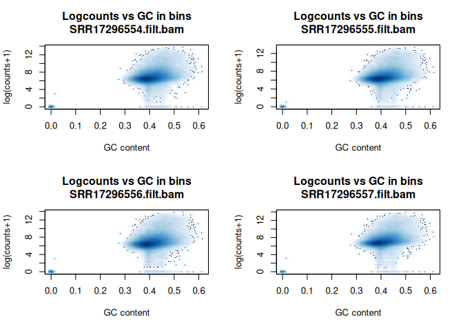
We can see that the signal of logcounts vs GC content looks very similar in all libraries.

5.2 GC Bias in Peaks

To ivestigate the GC bias in peaks (signal), we start with creating the GRanges object holding the peak intervals.

We need to prefix the chromosome name by “chr” (per UCSC convention) in the first step to be able to use a BSgenome object from the Bioconductor package BSgenome.Mmusculus.UCSC.mm39. Please note this only works with assembled chromosomes; the non-assembled contigs follow different naming conventions in Ensembl (the source of the reference assembly for read mapping) and UCSC (the source of BSgenome package).

peaks_gr=GRanges(seqnames=paste0("chr",cnt_table_chr$Chr), ranges=IRanges(cnt_table_chr$Start, cnt_table_chr$End), strand="*", mcols=data.frame(peakID=rownames(cnt_table_chr)))

We now prepare data with GC content of the peak regions for GC-aware normalisation.

peakSeqs=BSgenome::getSeq(Mmusculus,peaks_gr)

gcContentPeaks=Biostrings::letterFrequency(peakSeqs, "GC",as.prob=TRUE)[,1]

#divide into 20 bins by GC content
gcGroups=Hmisc::cut2(gcContentPeaks, g=20)
mcols(peaks_gr)$gc=gcContentPeaks
mcols(peaks_gr)$gc_group=gcGroups

peaks_gr
## GRanges object with 64879 ranges and 3 metadata columns:
##           seqnames            ranges strand |       mcols.peakID        gc
##              <Rle>         <IRanges>  <Rle> |        <character> <numeric>
##       [1]     chr1   3050939-3052959      * |     merged_peaks_1  0.392875
##       [2]     chr1   3053048-3054634      * |     merged_peaks_2  0.379962
##       [3]     chr1   3054861-3055532      * |     merged_peaks_3  0.345238
##       [4]     chr1   3057260-3057785      * |     merged_peaks_4  0.376426
##       [5]     chr1   3059375-3061360      * |     merged_peaks_5  0.402316
##       ...      ...               ...    ... .                ...       ...
##   [64875]     chrY 90814281-90815165      * | merged_peaks_64875  0.505085
##   [64876]     chrY 90815739-90816707      * | merged_peaks_64876  0.430341
##   [64877]     chrY 90818033-90819321      * | merged_peaks_64877  0.493406
##   [64878]     chrY 90819900-90820364      * | merged_peaks_64878  0.369892
##   [64879]     chrY 90821996-90824312      * | merged_peaks_64879  0.469141
##                gc_group
##                <factor>
##       [1] [0.234,0.396)
##       [2] [0.234,0.396)
##       [3] [0.234,0.396)
##       [4] [0.234,0.396)
##       [5] [0.396,0.417)
##       ...           ...
##   [64875] [0.505,0.514)
##   [64876] [0.417,0.431)
##   [64877] [0.487,0.496)
##   [64878] [0.234,0.396)
##   [64879] [0.461,0.470)
##   -------
##   seqinfo: 21 sequences from an unspecified genome; no seqlengths

Figure below shows that the accessibility measure of a particular genomic region is associated with its GC content. In this data set, the curves are almost identical for all samples, indicating no difference in GC bias between samples.

However, in some cases the slope and shape of the curves may differ between samples, which indicates that GC content effects are sample–specific and can therefore bias between–sample comparisons.

We start by creating a data frame with gc contents and read count in each peak in each sample as well as perform lowess (locally weighted scatterplot smoothing) regression to fit the trend:

lowListGC = list()
for(kk in 1:ncol(reads.peak)){
  set.seed(kk)
  lowListGC[[kk]] = lowess(x=gcContentPeaks, y=log1p(reads.peak[,kk]), f=1/10)
}

names(lowListGC)=colnames(reads.peak)

dfList = list()
for(ss in 1:length(lowListGC)){
  oox = order(lowListGC[[ss]]$x)
  dfList[[ss]] = data.frame(x=lowListGC[[ss]]$x[oox], y=lowListGC[[ss]]$y[oox], sample=names(lowListGC)[[ss]])
}
dfAll = do.call(rbind, dfList)
dfAll$sample = factor(dfAll$sample)

We can now plot the relationship of logcounts vs GC content:

plotGCHex = function(gr, counts){
  counts2=counts
  df=as_tibble(cbind(counts2,gc=mcols(gr)$gc))
  df=gather(df, sample, value, -gc)
  ggplot(data=df, aes(x=gc, y=log(value+1)) ) + 
    ylab("log(count + 1)") + xlab("GC-content") + 
    geom_hex(bins = 50) + theme_bw()
}

plot_GC_bias=plotGCHex(peaks_gr, rowMeans(reads.peak)) +
  theme(axis.title = element_text(size=16)) +
  labs(fill="Nr. of peaks") + 
  geom_line(aes(x=x, y=y, group=sample, color=sample), data=dfAll, linewidth=1) +
  scale_color_discrete()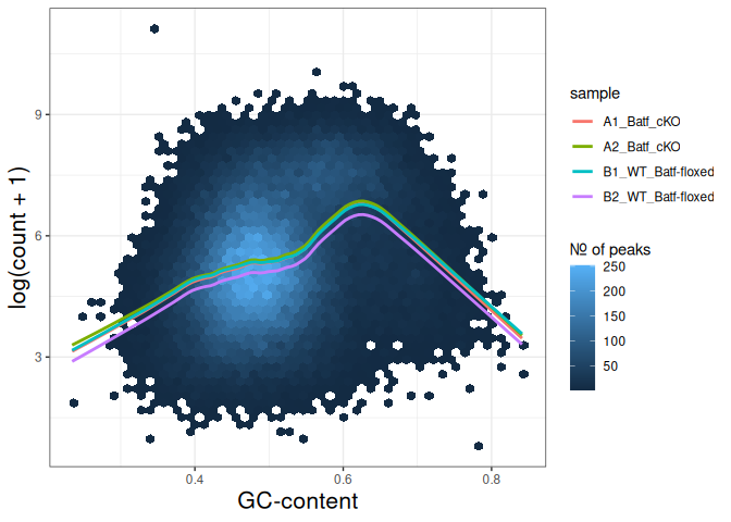

Figure 2: Fitted lowess curves of (non–normalised) logcounts as a function of GC content.

6 Differential Accessibility

We can define experimental groups:

groups=factor(c(rep("ctrl",2),rep("KO_Batf",2)))
groups
## [1] ctrl    ctrl    KO_Batf KO_Batf
## Levels: ctrl KO_Batf

design=model.matrix(~groups)
rownames(design)=colnames(reads.peak)
design
##                   (Intercept) groupsKO_Batf
## B1_WT_Batf-floxed           1             0
## B2_WT_Batf-floxed           1             0
## A1_Batf_cKO                 1             1
## A2_Batf_cKO                 1             1
## attr(,"assign")
## [1] 0 1
## attr(,"contrasts")
## attr(,"contrasts")$groups
## [1] "contr.treatment"

We will detect differentially accessible regions using edgeR. As we do not observe strong effects of GC content on signal neither in peaks nor in genomic bins, we decided to use the scaling normalisation by trimmed mean of M-values (TMM) (Robinson and Oshlack 2010).

We start by creating DGEList, the object edgeR uses to store data for calculations. Before we start the DA analysis, it is advisable to remove peaks with very low counts.

reads.dge = DGEList(counts=reads.peak, group=groups)
keep = filterByExpr(reads.dge)
reads.dge=reads.dge[keep,,keep.lib.sizes=FALSE]

summary(keep)
##    Mode   FALSE    TRUE 
## logical     418   64461

reads.dge
## An object of class "DGEList"
## $counts
##                B1_WT_Batf-floxed B2_WT_Batf-floxed A1_Batf_cKO A2_Batf_cKO
## merged_peaks_1               299               238         325         330
## merged_peaks_2               106                83         162         174
## merged_peaks_3                19                24          25          21
## merged_peaks_4                27                31          40          29
## merged_peaks_5               114               101          65         151
## 64456 more rows ...
## 
## $samples
##                     group lib.size norm.factors
## B1_WT_Batf-floxed    ctrl 43359738            1
## B2_WT_Batf-floxed    ctrl 33327965            1
## A1_Batf_cKO       KO_Batf 43438468            1
## A2_Batf_cKO       KO_Batf 46400831            1

These steps perform the standard edgeR workflow for differential analysis:

reads.dge.tmm = normLibSizes(reads.dge)

We can inspect sample grouping on multidimensional scaling (MDS) plot before proceeding:

plotMDS(reads.dge.tmm)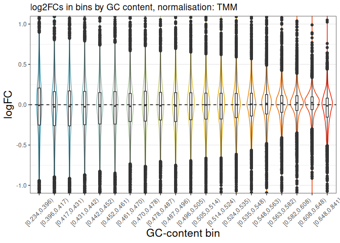

All looks as expected, we can proceed with the differential analysis:

reads.dge.tmm = estimateDisp(reads.dge.tmm, design)
qlf.fit.tmm = glmQLFit(reads.dge.tmm, design, robust=TRUE)
qlf.ftest.tmm = glmQLFTest(qlf.fit.tmm, coef=2)
DA_res.qlf.tmm = as.data.frame(topTags(qlf.ftest.tmm, nrow(qlf.ftest.tmm$table)))
DA_res.qlf.tmm = DA_res.qlf.tmm|>
  dplyr::mutate(peakID=rownames(DA_res.qlf.tmm))

This results in a table with results of DA analysis:

head(DA_res.qlf.tmm)

	logFC	logCPM	F	PValue	FDR	peakID
merged_peaks_28038	-1.610739	6.074221	753.7075	0	0	merged_peaks_28038
merged_peaks_51767	-1.508509	6.159745	711.1505	0	0	merged_peaks_51767
merged_peaks_2997	-1.517991	5.964106	636.4915	0	0	merged_peaks_2997
merged_peaks_1873	-1.157731	6.593339	530.8994	0	0	merged_peaks_1873
merged_peaks_36974	-1.141049	6.596216	523.9512	0	0	merged_peaks_36974
merged_peaks_40709	-1.638982	5.206780	470.4216	0	0	merged_peaks_40709

NoteDA results can be saved to a file as a table or rds object

write.table(DA_res.qlf.tmm, "Batf_WT_KO.merged_peaks.DA_TMM.tsv", 
    append = FALSE, 
    quote = FALSE, 
    sep = "\t",
    row.names = FALSE,
    col.names = TRUE, 
    fileEncoding = "")

saveRDS(DA_res.qlf.tmm, 
  file = "assets/rds/Batf_WT_KO.merged_peaks.DA_TMM.rds", 
  ascii = FALSE, 
  version = NULL, 
  compress = TRUE, 
  refhook = NULL)

We should also take a look at the diagnostic plots to verify that they look as expected.

plotMD(qlf.ftest.tmm)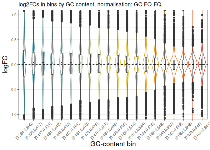

At this point we can add the information from peak annotation (../ATAC-peakAnnot/PeakAnnot.tsao2022.fulldata.14ix2026.html)

If you are still in the same R session, you can skip the step below.

If you started a new R session, you can read in the table with peak annotations:

peak_annots_pth=file.path("assets","rds","Batf_WT_KO.merged_peaks.annot.rds")

peakAnno_df=readRDS(peak_annots_pth)

#until cleaned up
peakAnno_df=peakAnno_df|>dplyr::rename(peakID=mcols.peakID)

We can now join the tables with peak annotations and DA results:

DA_res_table=DA_res.qlf.tmm |>
  dplyr::left_join(peakAnno_df,by="peakID")|>
  dplyr::select(seqnames,start,end,peakID,logFC,PValue,FDR,annotation,geneChr,geneStart,geneEnd,geneStrand,geneId,transcriptId,external_gene_name,distanceToTSS)|>
  dplyr::mutate(annotation=str_replace_all(annotation,  " \\s*\\([^\\)]+\\)", ""))

head(DA_res_table)

seqnames	start	end	peakID	logFC	PValue	FDR	annotation	geneChr	geneStart	geneEnd	geneStrand	geneId	transcriptId	external_gene_name	distanceToTSS
17	66268427	66269247	merged_peaks_28038	-1.610739	0	0	Distal Intergenic	17	66261129	66265392	1	ENSMUSG00000139744	ENSMUST00000355127	Gm65735	7298
6	122504236	122505014	merged_peaks_51767	-1.508509	0	0	Intron	6	122499458	122505594	1	ENSMUSG00000030116	ENSMUST00000126357	Mfap5	4778
1	155076669	155077704	merged_peaks_2997	-1.517991	0	0	3’ UTR	1	155070767	155077993	1	ENSMUSG00000026470	ENSMUST00000194158	Stx6	5902
1	95195320	95196614	merged_peaks_1873	-1.157731	0	0	Distal Intergenic	1	95183688	95184535	2	ENSMUSG00000099592	ENSMUST00000190584	Gm5264	-10785
2	162944874	162945676	merged_peaks_36974	-1.141049	0	0	Distal Intergenic	2	162934819	162934943	1	ENSMUSG00002076785	ENSMUST00020181897	Gm56299	10055
3	138125917	138126743	merged_peaks_40709	-1.638982	0	0	Exon	3	138121256	138136653	1	ENSMUSG00000037797	ENSMUST00000013458	Adh4	4661

saveRDS(DA_res_table, 
  file = "assets/rds/Batf_WT_KO.merged_peaks.DA_TMM.annot.rds", 
  ascii = FALSE, 
  version = NULL, 
  compress = TRUE, 
  refhook = NULL)

7 GC Bias Correction

7.1 Plotting Log2FC in GC Bins

When a strong effect of GC content on signal is observed, a GC aware scaling normalisation can be considered. It is important to perform all diagnostic plots, however, to verify whether it does not distort the data in an unexpected manner. One should always be aware that the GC bias, although technical, may also reflect sample biology, therefore removing it may lead to signal loss.

We can first verify whether there is a GC bias in log2FC detection using GC agnostic TMM scaling.

We can plot log2FC distribution in GC content bins.

For this we will need the GC bins we calculated before, so we need to join that information to the results of DA analysis:

peak_info_df=as.data.frame(peaks_gr)|>
  dplyr::rename(peakID=mcols.peakID)

df_GCbias=DA_res.qlf.tmm |>
    dplyr::left_join(peak_info_df, by="peakID") |>
    dplyr::select(logFC,gc_group)

We can plot the log2FC in GC bins:

plot_lfc_GC_TMM = ggplot(df_GCbias) +
  aes(x=gc_group, y=logFC, color=gc_group) +
  geom_violin(width=0.95) +
  geom_boxplot(width=0.15, color="grey20") +
  scale_color_manual(values=wesanderson::wes_palette("Zissou1", nlevels(df_GCbias$gc_group), "continuous")) +
  geom_abline(intercept = 0, slope = 0, col="black", lty=2) +
  #ylim(c(-1,1)) + ## this was in the original code from EDAseq paper; it calculates medians for values within the ylim interval - not from the entire data
  coord_cartesian(ylim=c(-1,1)) +
  ggtitle(paste0("log2FCs in bins by GC content, normalisation: TMM")) +
  xlab("GC-content bin") +
  theme_bw()+
  theme(axis.text.x = element_text(angle = 45, vjust = .5),
        legend.position = "none",
        axis.title = element_text(size=16))

plot_lfc_GC_TMM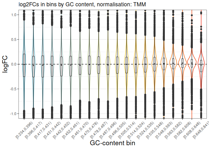

In this case a negligible bias in log2FC can be observed within the range of log2FC (-1,1).

You can alter the plotted range by changing coord_cartesian(ylim=c(-1,1)) to your desired range.

In any case, for this data set the systematic effect of GC contents on detected log2FC is very small, and below the reasonable size effect cutoff.

7.2 Correcting for GC contents

If required, the raw counts can be scaled in a GC aware manner, rather than using the TMM method.

Two related methods are presented below. Both perform conditional quantile scaling, and output the offsets which can then be used in edgeR statistical framework.

7.2.1 Full Quantile GC-GC Scaling

This method is implemented in Bioconductor package EDASeq (Risso et al. 2011).

To calculate the offsets, which correct for library size as well as GC content (full quantile normalisation in both cases):

exprsSet.eda=newSeqExpressionSet(reads.dge$counts)
peaks_gr.keep=peaks_gr[keep]
fData(exprsSet.eda)$gc=peaks_gr.keep$gc

exprsSet.eda.wl=withinLaneNormalization(exprsSet.eda,"gc",num.bins=20, which="full",offset=TRUE)
exprsSet.eda.bl=betweenLaneNormalization(exprsSet.eda.wl,which="full",offset=TRUE)

These peak and library level offsets can be inspected:

head(offst(exprsSet.eda.bl))
##                B1_WT_Batf-floxed B2_WT_Batf-floxed A1_Batf_cKO A2_Batf_cKO
## merged_peaks_1         1.2280870         1.5061165   1.2441529   1.1811897
## merged_peaks_2         1.0093249         1.2584039   1.1587582   1.0848913
## merged_peaks_3         0.6129416         0.9425809   0.7350182   0.5523253
## merged_peaks_4         0.7139578         0.9909705   0.8238461   0.6286266
## merged_peaks_5         0.6563096         0.9560009   0.5779452   0.6904069
## merged_peaks_6         0.6932922         1.0369034   0.7632731   0.7825120

We will input the offset to edgeR:

reads.dge.edaseq = reads.dge
reads.dge.edaseq$offset = -offst(exprsSet.eda.bl)

The statistical testing follows:

reads.dge.edaseq=estimateDisp(reads.dge.edaseq, design)
qlf.fit.edaseq=glmQLFit(reads.dge.edaseq, design, robust=TRUE)
qlf.ftest.edaseq=glmQLFTest(qlf.fit.edaseq, coef=2)
DA_res.qlf.edaseq=as.data.frame(topTags(qlf.ftest.edaseq, nrow(qlf.ftest.edaseq$table)))
DA_res.qlf.edaseq=DA_res.qlf.edaseq|>dplyr::mutate(peakID=rownames(DA_res.qlf.edaseq))

We can now plot the log2FC in GC bins, as for TMM scaling:

df_GCbias=DA_res.qlf.edaseq |>
    dplyr::left_join(peak_info_df, by="peakID") |>
    dplyr::select(logFC,gc_group)

plot_lfc_GC_edaseq = ggplot(df_GCbias) +
  aes(x=gc_group, y=logFC, color=gc_group) +
  geom_violin(width=0.95) +
  geom_boxplot(width=0.15, color="grey20") +
  scale_color_manual(values=wesanderson::wes_palette("Zissou1", nlevels(df_GCbias$gc_group), "continuous")) +
  geom_abline(intercept = 0, slope = 0, col="black", lty=2) +
  #ylim(c(-1,1)) + ## this was in the original code from EDAseq paper; it calculates medians for values within the ylim interval - not from the entire data
  coord_cartesian(ylim=c(-1,1)) +
  ggtitle(paste0("log2FCs in bins by GC content, normalisation: GC FQ-FQ")) +
  xlab("GC-content bin") +
  theme_bw()+
  theme(axis.text.x = element_text(angle = 45, vjust = .5),
        legend.position = "none",
        axis.title = element_text(size=16))

plot_lfc_GC_edaseq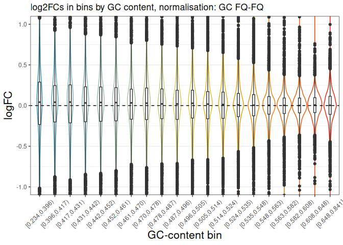

7.2.2 Conditional Quantile Normalization

This method is implemented in Bioconductor package cqn (Hansen et al. 2012).

In calculating offsets, it can correct both for GC content as well as peak length.

#assuming we have the subset peaks_gr
peaks_gr.keep=peaks_gr[keep]


peaks=as.data.frame(cbind(
      gc=peaks_gr.keep$gc,
      length=width(peaks_gr.keep)
    ))
rownames(peaks)=peaks_gr.keep$mcols.peakID

cqn_out=cqn(counts=reads.dge$counts,lengths=peaks$length,x=peaks$gc,
             sizeFactors=reads.dge$samples$lib.size,verbose=TRUE)
## RQ fit ....
## SQN
## .

cqn_out
## 
## Call:
##  cqn(counts = reads.dge$counts, x = peaks$gc, lengths = peaks$length, 
##     sizeFactors = reads.dge$samples$lib.size, verbose = TRUE) 
## 
## Object of class 'cqn' with
##   64461 regions
##   4 samples
## fitted using smooth length

head(cqn_out$glm.offset)
##                B1_WT_Batf-floxed B2_WT_Batf-floxed A1_Batf_cKO A2_Batf_cKO
## merged_peaks_1          6.077630          5.849091    6.038654    6.142638
## merged_peaks_2          5.602194          5.392023    5.695700    5.805515
## merged_peaks_3          3.810420          3.669992    3.829517    3.872245
## merged_peaks_4          3.460506          3.172147    3.333104    3.457118
## merged_peaks_5          5.812975          5.660115    5.655834    6.000880
## merged_peaks_6          5.993356          5.874478    5.930493    6.225818

We will input the offset to edgeR:

reads.dge.cqn = reads.dge
reads.dge.cqn$offset = cqn_out$glm.offset

The statistical testing follows:

reads.dge.cqn=estimateDisp(reads.dge.cqn, design)
qlf.fit.cqn=glmQLFit(reads.dge.cqn, design, robust=TRUE)
qlf.ftest.cqn=glmQLFTest(qlf.fit.cqn, coef=2)
DA_res.qlf.cqn=as.data.frame(topTags(qlf.ftest.cqn, nrow(qlf.ftest.cqn$table)))
DA_res.qlf.cqn=DA_res.qlf.cqn|>dplyr::mutate(peakID=rownames(DA_res.qlf.cqn))

We can now plot the log2FC in GC bins, as for TMM scaling:

df_GCbias=DA_res.qlf.cqn |>
    dplyr::left_join(peak_info_df, by="peakID") |>
    dplyr::select(logFC,gc_group)

plot_lfc_GC_cqn = ggplot(df_GCbias) +
  aes(x=gc_group, y=logFC, color=gc_group) +
  geom_violin(width=0.95) +
  geom_boxplot(width=0.15, color="grey20") +
  scale_color_manual(values=wesanderson::wes_palette("Zissou1", nlevels(df_GCbias$gc_group), "continuous")) +
  geom_abline(intercept = 0, slope = 0, col="black", lty=2) +
  #ylim(c(-1,1)) + ## this was in the original code from EDAseq paper; it calculates medians for values within the ylim interval - not from the entire data
  coord_cartesian(ylim=c(-1,1)) +
  ggtitle(paste0("log2FCs in bins by GC content, normalisation: cqn")) +
  xlab("GC-content bin") +
  theme_bw()+
  theme(axis.text.x = element_text(angle = 45, vjust = .5),
        legend.position = "none",
        axis.title = element_text(size=16))

plot_lfc_GC_cqn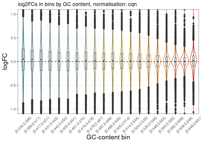

Note

It is advised to verify the estimated model parameters and fit using the diagnostic plots provided in edgeR i.e. plotBCV(reads.dge) and plotQLDisp(fit)

8 Session Info

NoteSession Info

sessionInfo()
## R version 4.6.1 (2026-06-24)
## Platform: x86_64-pc-linux-gnu
## Running under: Ubuntu 24.04.5 LTS
## 
## Matrix products: default
## BLAS:   /usr/lib/x86_64-linux-gnu/openblas-pthread/libblas.so.3 
## LAPACK: /usr/lib/x86_64-linux-gnu/openblas-pthread/libopenblasp-r0.3.26.so;  LAPACK version 3.12.0
## 
## locale:
##  [1] LC_CTYPE=C.UTF-8       LC_NUMERIC=C           LC_TIME=C.UTF-8       
##  [4] LC_COLLATE=C.UTF-8     LC_MONETARY=C.UTF-8    LC_MESSAGES=C.UTF-8   
##  [7] LC_PAPER=C.UTF-8       LC_NAME=C              LC_ADDRESS=C          
## [10] LC_TELEPHONE=C         LC_MEASUREMENT=C.UTF-8 LC_IDENTIFICATION=C   
## 
## time zone: UTC
## tzcode source: system (glibc)
## 
## attached base packages:
## [1] stats4    stats     graphics  grDevices datasets  utils     methods  
## [8] base     
## 
## other attached packages:
##  [1] cqn_1.58.0                         mclust_6.1.3                      
##  [3] EDASeq_2.46.0                      ShortRead_1.70.0                  
##  [5] GenomicAlignments_1.48.0           Rsamtools_2.28.0                  
##  [7] BiocParallel_1.46.0                SummarizedExperiment_1.42.0       
##  [9] Biobase_2.72.0                     MatrixGenerics_1.24.0             
## [11] matrixStats_1.5.0                  edgeR_4.10.3                      
## [13] limma_3.68.5                       BSgenome.Mmusculus.UCSC.mm39_1.4.3
## [15] BSgenome_1.80.0                    rtracklayer_1.72.0                
## [17] BiocIO_1.22.0                      MASS_7.3-65                       
## [19] regioneR_1.44.0                    Biostrings_2.80.0                 
## [21] XVector_0.52.0                     Hmisc_5.3-0                       
## [23] GenomicRanges_1.64.0               Seqinfo_1.2.0                     
## [25] IRanges_2.46.0                     S4Vectors_0.50.2                  
## [27] BiocGenerics_0.58.1                generics_0.1.4                    
## [29] wesanderson_0.3.7                  kableExtra_1.4.1                  
## [31] lubridate_1.9.5                    forcats_1.0.1                     
## [33] stringr_1.6.0                      dplyr_1.2.1                       
## [35] purrr_1.2.2                        readr_2.2.0                       
## [37] tidyr_1.3.2                        tibble_3.3.1                      
## [39] ggplot2_4.0.3                      tidyverse_2.0.0                   
## [41] knitr_1.51                        
## 
## loaded via a namespace (and not attached):
##   [1] splines_4.6.1          bitops_1.0-9           filelock_1.0.3        
##   [4] R.oo_1.27.1            XML_3.99-0.23          rpart_4.1.27          
##   [7] lifecycle_1.0.5        httr2_1.2.2            pwalign_1.8.0         
##  [10] lattice_0.22-9         backports_1.5.1        magrittr_2.0.5        
##  [13] rmarkdown_2.31         yaml_2.3.12            otel_0.2.0            
##  [16] DBI_1.3.0              RColorBrewer_1.1-3     abind_1.4-8           
##  [19] R.utils_2.13.0         RCurl_1.98-1.18        nnet_7.3-20           
##  [22] rappdirs_0.3.4         MatrixModels_0.5-4     svglite_2.2.2         
##  [25] codetools_0.2-20       DelayedArray_0.38.1    xml2_1.6.0            
##  [28] tidyselect_1.2.1       UCSC.utils_1.8.0       farver_2.1.2          
##  [31] BiocFileCache_3.2.0    base64enc_0.1-6        jsonlite_2.0.0        
##  [34] Formula_1.2-6          survival_3.8-6         systemfonts_1.3.2     
##  [37] tools_4.6.1            progress_1.2.3         Rcpp_1.1.1-1.1        
##  [40] glue_1.8.1             gridExtra_2.3.1        SparseArray_1.12.2    
##  [43] xfun_0.57              GenomeInfoDb_1.48.0    withr_3.0.2           
##  [46] BiocManager_1.30.27    fastmap_1.2.0          latticeExtra_0.6-31   
##  [49] SparseM_1.84-2         digest_0.6.39          timechange_0.4.0      
##  [52] R6_2.6.1               textshaping_1.0.5      colorspace_2.1-2      
##  [55] jpeg_0.1-11            dichromat_2.0-1        biomaRt_2.68.0        
##  [58] RSQLite_3.53.1         cigarillo_1.2.0        R.methodsS3_1.8.2     
##  [61] hexbin_1.28.6          renv_1.2.3             data.table_1.18.6.1   
##  [64] prettyunits_1.2.0      httr_1.4.8             htmlwidgets_1.6.4     
##  [67] S4Arrays_1.12.0        pkgconfig_2.0.3        gtable_0.3.6          
##  [70] blob_1.3.0             S7_0.2.2               hwriter_1.3.2.1       
##  [73] htmltools_0.5.9        scales_1.4.0           png_0.1-9             
##  [76] rstudioapi_0.19.0      tzdb_0.5.0             rjson_0.2.23          
##  [79] checkmate_2.3.4        curl_7.1.0             cachem_1.1.0          
##  [82] KernSmooth_2.23-26     parallel_4.6.1         foreign_0.8-91        
##  [85] AnnotationDbi_1.74.0   restfulr_0.0.16        pillar_1.11.1         
##  [88] grid_4.6.1             vctrs_0.7.3            dbplyr_2.5.2          
##  [91] cluster_2.1.8.2        htmlTable_2.5.0        evaluate_1.0.5        
##  [94] GenomicFeatures_1.64.0 cli_3.6.6              locfit_1.5-9.12       
##  [97] compiler_4.6.1         rlang_1.3.0            crayon_1.5.3          
## [100] labeling_0.4.3         nor1mix_1.3-3          interp_1.1-6          
## [103] aroma.light_3.42.0     stringi_1.8.7          viridisLite_0.4.3     
## [106] deldir_2.0-4           quantreg_6.1           Matrix_1.7-5          
## [109] hms_1.1.4              bit64_4.8.2            KEGGREST_1.52.0       
## [112] statmod_1.5.2          memoise_2.0.1          bit_4.6.0

9 References

Chen, Yunshun, Aaron T. L. Lun, and Gordon K. Smyth. 2016. “From Reads to Genes to Pathways: Differential Expression Analysis of RNA-Seq Experiments Using Rsubread and the edgeR Quasi-Likelihood Pipeline.” F1000Research 5 (August): 1438. https://doi.org/10.12688/f1000research.8987.2.

Hansen, K. D., R. A. Irizarry, and Z. WU. 2012. “Removing Technical Variability in RNA-Seq Data Using Conditional Quantile Normalization.” Biostatistics 13 (2): 204–16. https://doi.org/10.1093/biostatistics/kxr054.

Risso, Davide, Katja Schwartz, Gavin Sherlock, and Sandrine Dudoit. 2011. “GC-Content Normalization for RNA-Seq Data.” BMC Bioinformatics 12 (1). https://doi.org/10.1186/1471-2105-12-480.

Robinson, M. D., and A. Oshlack. 2010. “A scaling normalization method for differential expression analysis of RNA-seq data.” Genome Biol 11 (3): R25.

Tsao, Hsiao-Wei, James Kaminski, Makoto Kurachi, et al. 2022. “Batf-Mediated Epigenetic Control of Effector CD8 + t Cell Differentiation.” Science Immunology 7 (68). https://doi.org/10.1126/sciimmunol.abi4919.