Mathematical statistics and machine learning in R
RaukR 2024 • Advanced R for Bioinformatics
21-Jun-2024
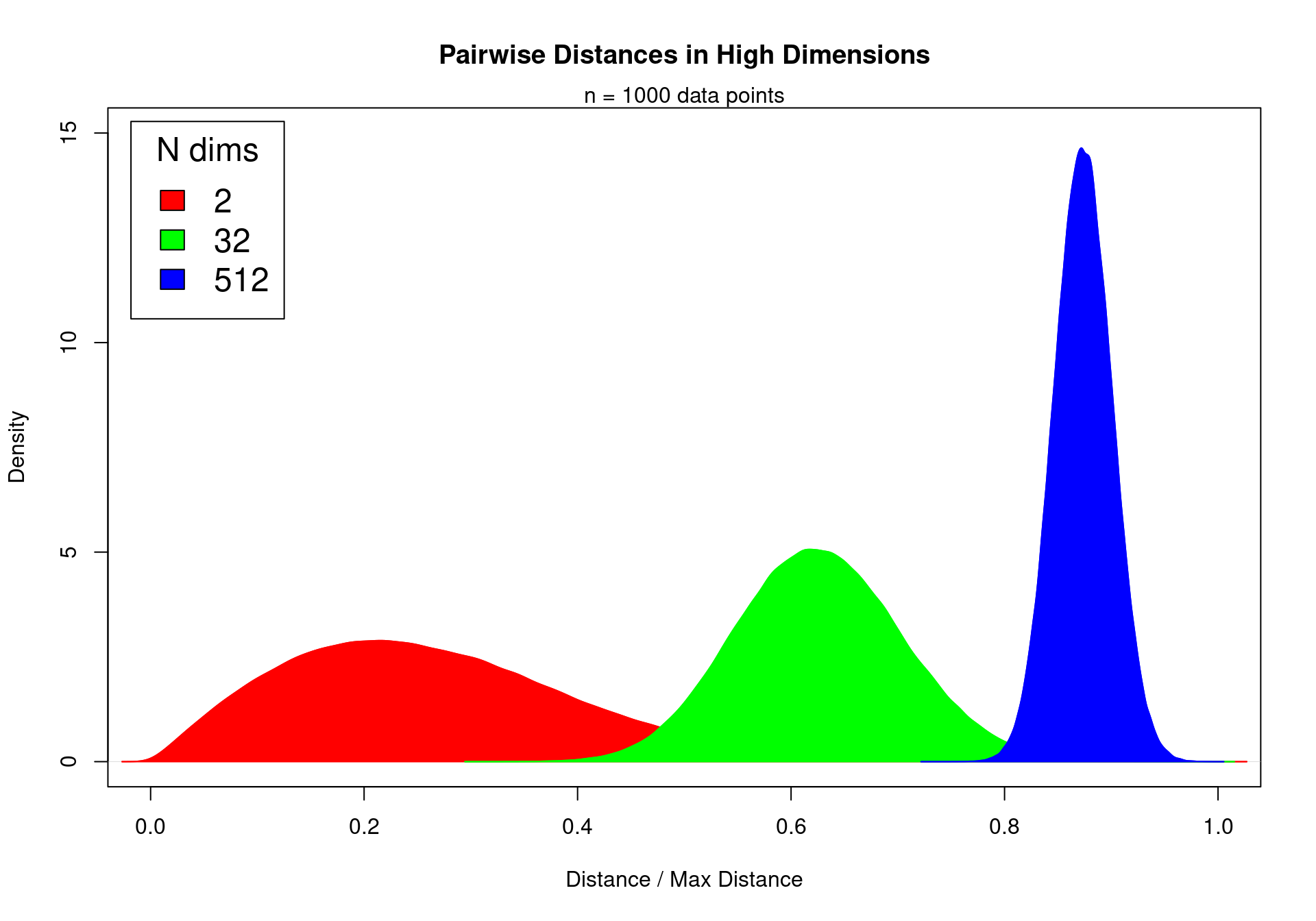
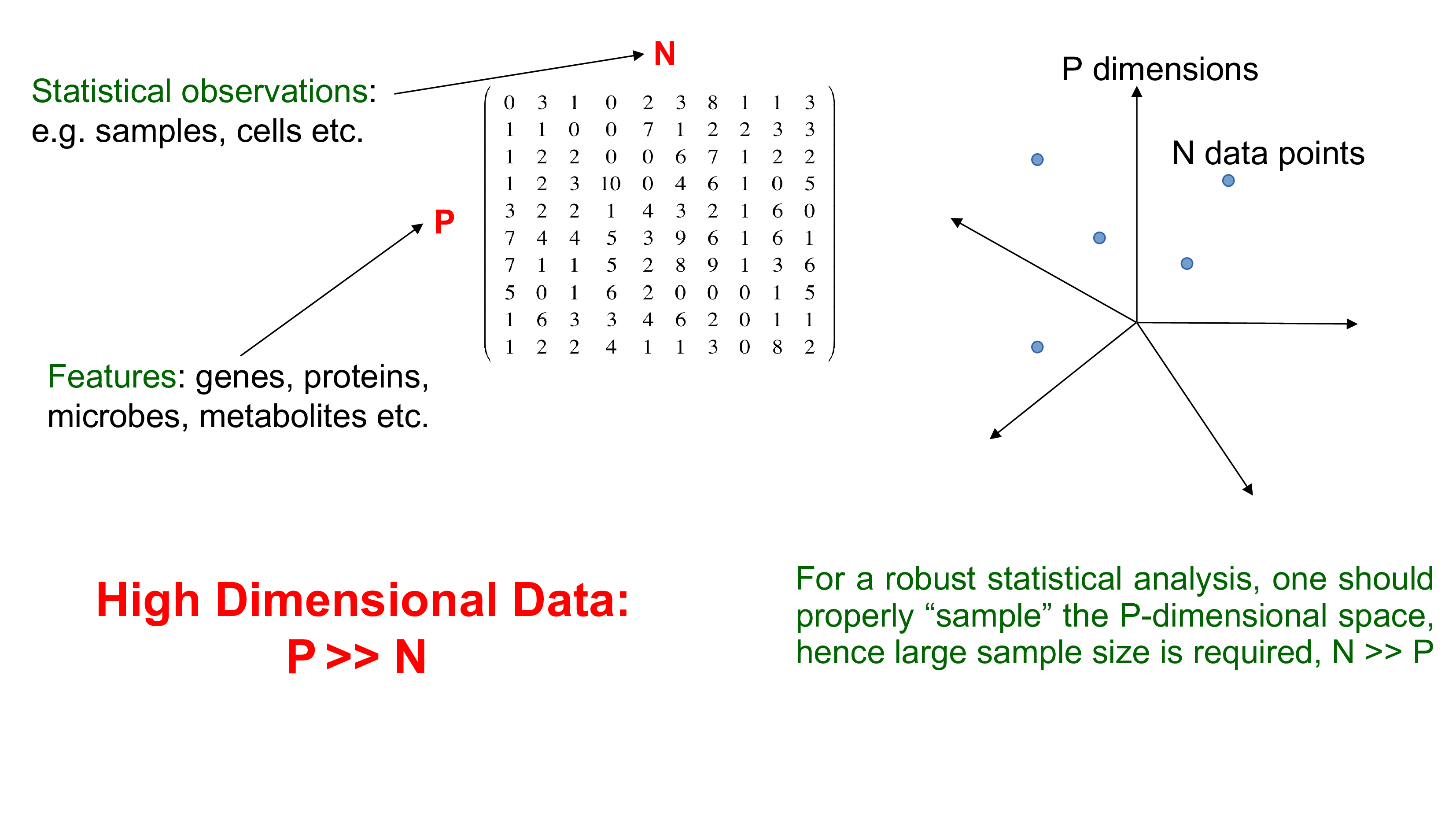
Biological data are high dimensional
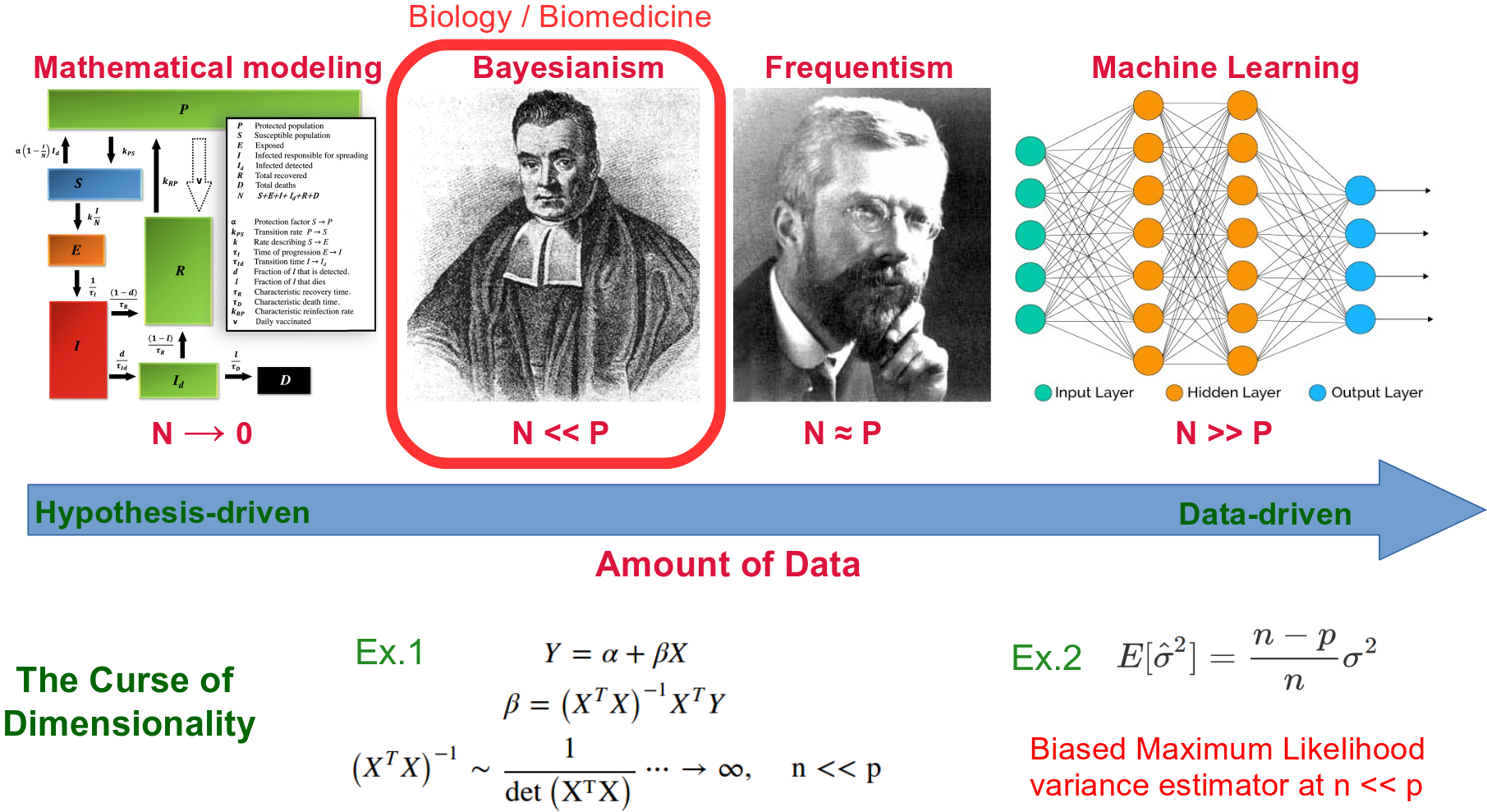
Types of data analysis
Some peculiarities of Frequentist statistics
- based on Maximum Likelihood principle
- focus
too muchon summary statistics
\[\rm{L}\,(\,x_i \,|\, \mu,\sigma^2\,) = \frac{1}{\sqrt{2\pi\sigma^2}} \exp^{\displaystyle -\frac{\sum\limits_{i=1}^N (x_i-\mu)^2}{2\sigma^2}}\]
\[\frac{\partial \rm{L}\,(\,x_i \,|\, \mu,\sigma^2\,)}{\partial\mu} = 0; \,\, \frac{\partial \rm{L}\,(\,x_i \,|\, \mu,\sigma^2\,)}{\partial\sigma^2} = 0\]
\[\mu = \frac{1}{N}\sum_{i=0}^N x_i \,\,\rm{-}\,\rm{mean \, estimator}\]
\[\sigma^2 = \frac{1}{N}\sum_{i=0}^N (x_i-\mu)^2 \,\,\rm{-}\,\rm{variance \, estimator}\]
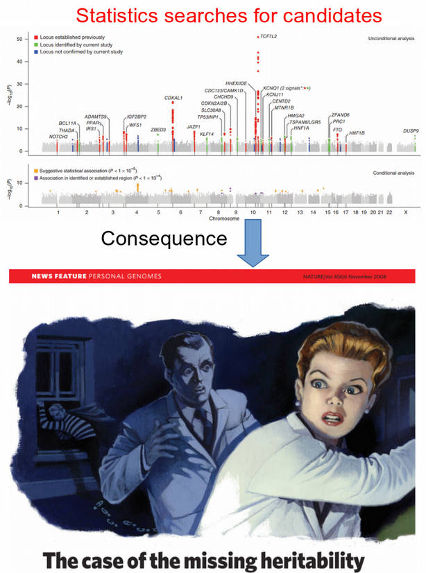
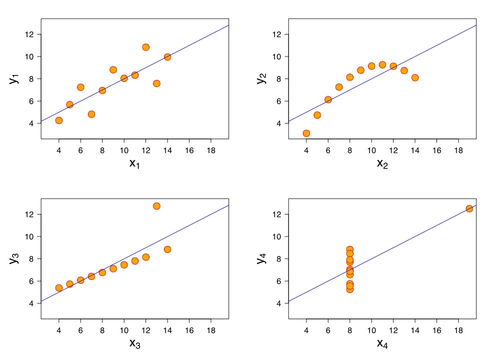 Summary statistics do not always reasonbly describe data (example: Anscombes quartet)
Frequentist statistics: focus to much on p-values
FC<-1.02; x_mean<-5; x_sd<-1; N_vector<-seq(from=100,to=10000,by=100); pvalue_t<-vector(); pvalue_lm<-vector()
for(N in N_vector)
{
  x1 <- rnorm(N, x_mean, x_sd); x2 <- rnorm(N, x_mean*FC, x_sd)
  t_test_res<-t.test(x1, x2); pvalue_t <- append(pvalue_t, t_test_res$p.value)

  x <- rnorm(N, 0, 1); y <- 0.1*x+2*rnorm(N, 0, 1)
  lm_res <- summary(lm(y~x)); pvalue_lm <- append(pvalue_lm, lm_res$coefficients[2,4])
}
par(mfrow=c(2,2)); par(mar = c(5, 5, 1, 1))
boxplot(x1, x2, names=c("X1","X2"), ylab="Value", col="darkred"); mtext("Fold change FC = 1.02")
plot(pvalue_t~N_vector,type='o',xlab="N",ylab="p-value",col="darkgreen"); mtext("P-value of two-group t-test")
plot(y~x, xlab="X", ylab="Y"); abline(lm(y~x), col="blue", lwd=2); mtext("Y = 0.1*X + 2*rnorm(N, 0, 1)")
plot(pvalue_lm~N_vector,type='o',xlab="N",ylab="p-value",col="darkgreen"); mtext("P-value of linear regression")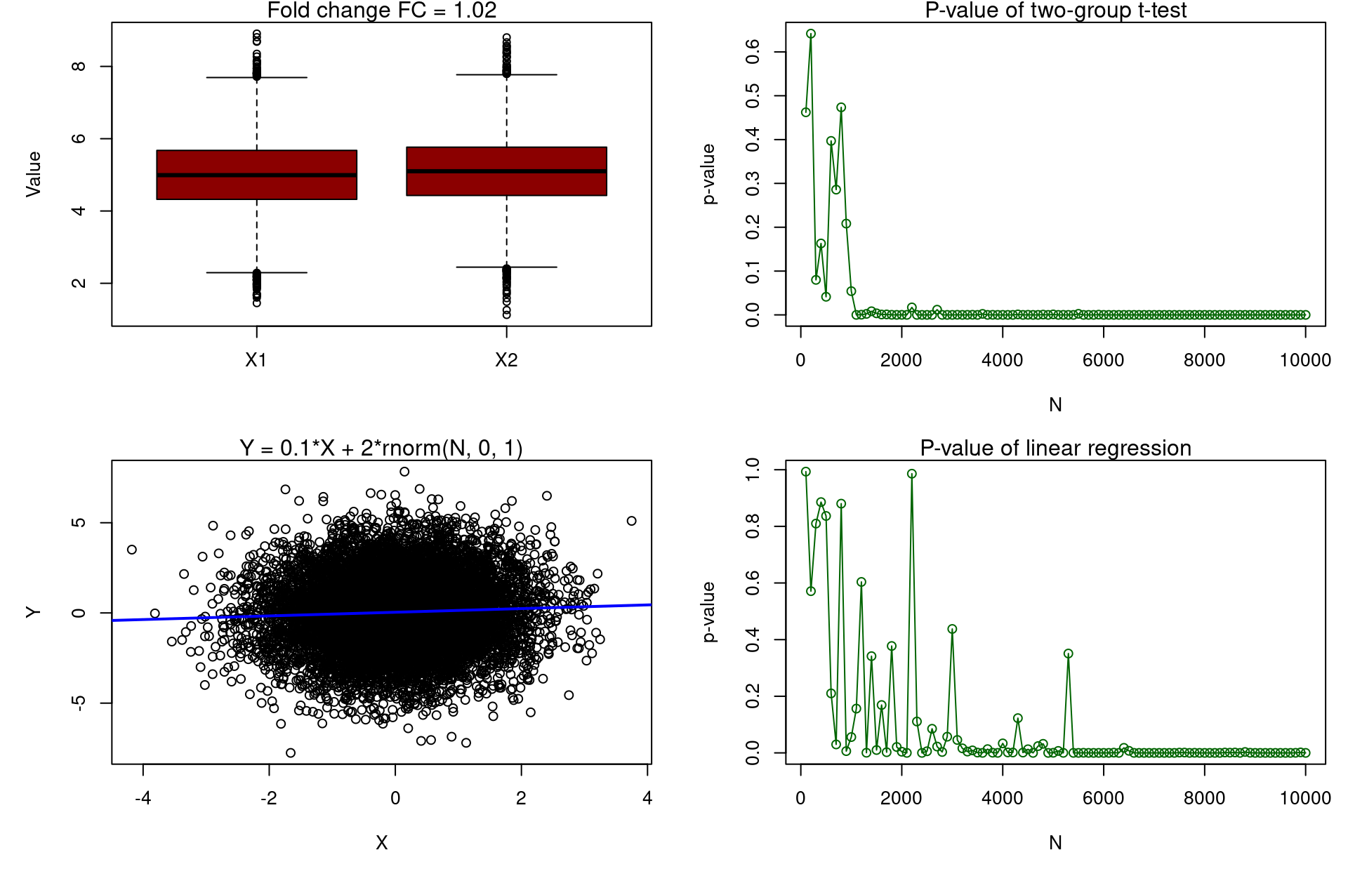

Questionable whether p-value is a best metric for ranking features (biomarkers)
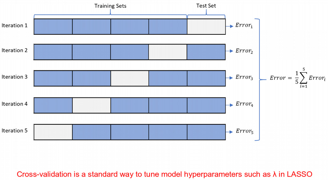
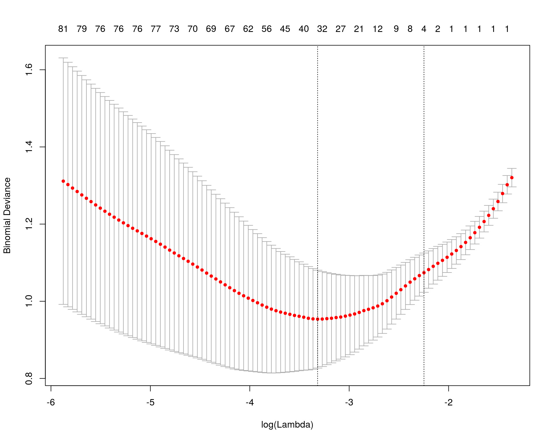
Regularizations: LASSO
\[Y = \beta_1X_1+\beta_2X_2+\epsilon\]
\[\textrm{OLS} = (Y-\beta_1X_1-\beta_2X_2)^2\]
\[\textrm{Penalized OLS} = (Y-\beta_1X_1-\beta_2X_2)^2 + \lambda(|\beta_1|+|\beta_2|)\]
Markov Chain Monte Carlo (MCMC): introduction
- Integration via Monte Carlo sampling
\[\small I = 2\int\limits_2^4{x dx}=2\frac{x^2}{2} \Big|_2^4 = 16 - 4 = 12\]
f <- function(x){return(2*x)}; a <- 2; b <- 4; N <- 10000; count <- 0
x <- seq(from = a, to = b, by = (b-a) / N); y_max <- max(f(x))
for(i in 1:N)
{
  x_sample <- runif(1, a, b); y_sample <- runif(1, 0, y_max)
  if(y_sample <= f(x_sample)){count <- count + 1}
}
paste0("Integral by Monte Carlo: I = ", (count / N) * (b - a) * y_max)
[1] "Integral by Monte Carlo: I = 11.9248"- Markov Chain Monte Carlo (MCMC)
\[\small \rm{Hastings \,\, ratio} = \frac{\rm{Posterior}\,(\,\rm{params_{next}} \,|\, \rm{data}\,)}{\rm{Posterior}\,(\,\rm{params_{previous}} \,|\, \rm{data}\,)}\]
- If Hastings ratio > u [0, 1], then accept, else reject
- Hastings ratio does not contain the intractable integral from Bayes theorem
Markov Chain Monte Carlo (MCMC) from scratch in R
- Example from population genetics
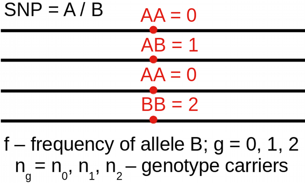
\[\small L(n \, | \, f) = \prod_g{\left[ {2\choose g} f^g (1-f)^{2-g} \right]^{n_g}}\]
\[\small \frac{\partial \log\left[L(n | f)\right]}{\partial f} = 0 \, \Rightarrow \hat{f}=\frac{n_1+2n_2}{2(n_0+n_1+n_2)}\]
\[\small \rm{Prior}(f, \alpha, \beta) = \frac{1}{B(\alpha, \beta)} f^{\alpha-1} (1-f)^{\beta-1}\]
N <- 100; n <- c(25, 50, 25) # Observed genotype data for N individuals
f_MLE <- (n[2] + 2*n[3]) / (2 * sum(n)) # MLE of allele frequency
# Define log-likelihood function (log-binomial distribution)
LL <- function(n, f){return((n[2] + 2*n[3])*log(f) + (n[2] + 2*n[1])*log(1-f))}
# Define log-prior function (log-beta distribution)
LP <- function(f, alpha, beta){return(dbeta(f, alpha, beta, log = TRUE))}
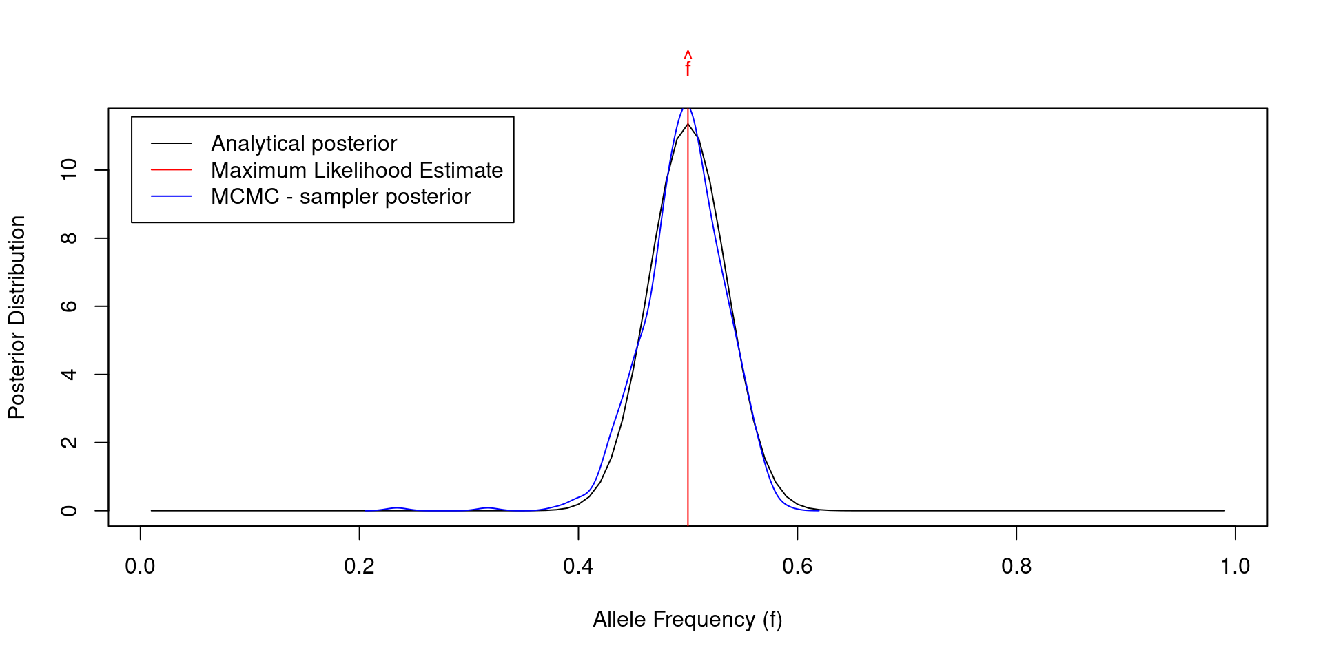
# Run MCMC Metropolis - Hastings sampler
f_poster <- vector(); alpha <- 0.5; beta <- 0.5; f_cur <- 0.1 # initialization
for(i in 1:1000)
{
f_next <- abs(rnorm(1, f_cur, 0.1)) # make random step for allele frequency
LL_cur <- LL(n, f_cur); LL_next <- LL(n, f_next)
LP_cur <- LP(f_cur, alpha, beta); LP_next <- LP(f_next, alpha, beta)
hastings_ratio <- LL_next + LP_next - LL_cur - LP_cur
if(hastings_ratio > log(runif(1))){f_cur <- f_next}; f_poster[i] <- f_cur
}
Moving from statistics to machine learning
- Statistics is more analytical (pen & paper)
\[\rm{L}\,(\,x_i \,|\, \mu,\sigma^2\,) = \frac{1}{\sqrt{2\pi\sigma^2}} \exp^{\displaystyle -\frac{\sum\limits_{i=1}^N (x_i-\mu)^2}{2\sigma^2}}\]
\[\frac{\partial \rm{L}\,(\,x_i \,|\, \mu,\sigma^2\,)}{\partial\mu} = 0; \,\, \frac{\partial \rm{L}\,(\,x_i \,|\, \mu,\sigma^2\,)}{\partial\sigma^2} = 0\]
\[\mu = \frac{1}{N}\sum_{i=0}^N x_i \,\,\rm{-}\,\rm{mean \, estimator}\]
\[\sigma^2 = \frac{1}{N}\sum_{i=0}^N (x_i-\mu)^2 \,\,\rm{-}\,\rm{variance \, estimator}\]
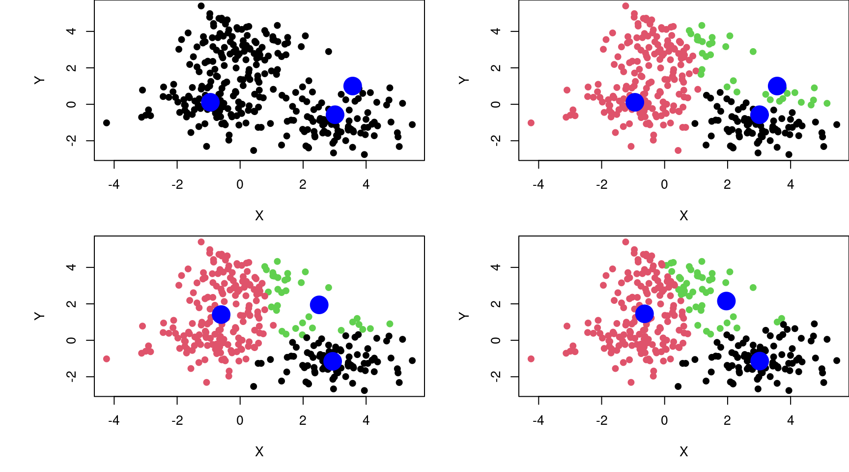
- Machine Learning is more algorithmic (ex. K-means)
K = 3; set.seed(123); c = X[sample(1:dim(X)[1],K),]; par(mfrow=c(2,2),mai=c(0.8,1,0,0))
plot(X, xlab = "X", ylab = "Y", pch = 19); points(c, col = "blue", cex = 3, pch = 19)
for(t in 1:3)
{
  l <- vector()
  for(i in 1:dim(X)[1])
  {
    d <- vector(); for(j in 1:K){d[j] <- sqrt((X[i,1]-c[j,1])^2 + (X[i,2]-c[j,2])^2)}
    l[i] <- which.min(d)
  }
  plot(X, xlab="X", ylab="Y", col=l, pch=19); points(c, col="blue", cex=3, pch=19)
  s = list(); for(i in unique(l)){s[[i]] <- colMeans(X[l==i,])}; c = Reduce("rbind", s)
}
Statistics vs. machine learning: prediction

How does machine learning work?
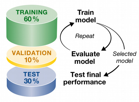
Machine Learning typically involves five basic steps:
1. Split data set into train, validation and test subsets
- Fit the model on the train subset
- Validate your model on the validation subset
- Repeat train - validation split many times and tune hyperparameters
- Test the accuracy of the optimized model on the test subset.
Toy example of machine learning
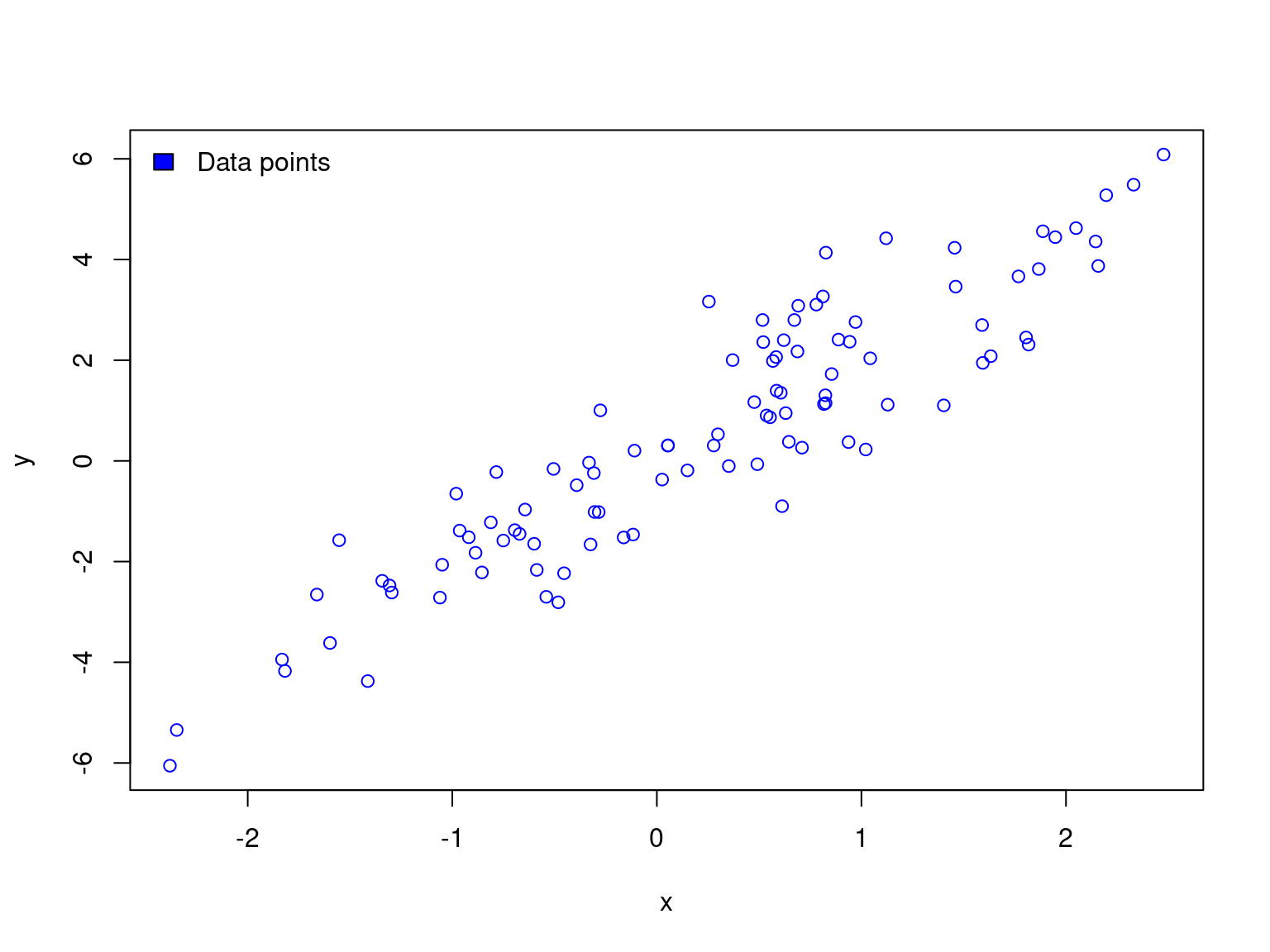
train <- df[sample(1:dim(df)[1], 0.7 * dim(df)[1]), ]
test <- df[!rownames(df) %in% rownames(train), ]
df$col <- ifelse(rownames(df) %in% rownames(test), "red", "blue")
plot(y ~ x, data = df, col = df$col)
legend("topleft", c("Train","Test"), fill=c("blue","red"), bty="n")
abline(lm(y ~ x, data = train), col = "blue")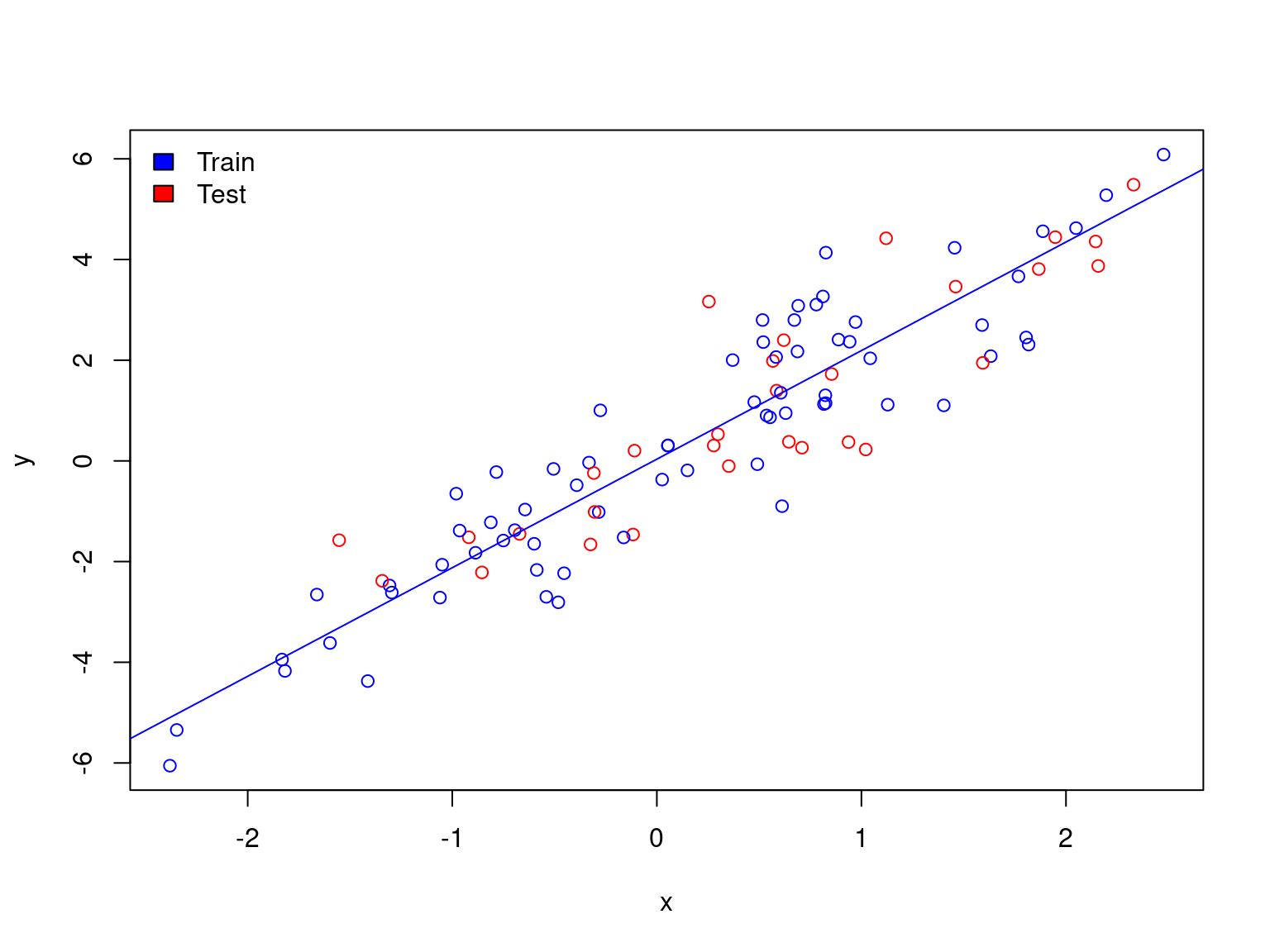
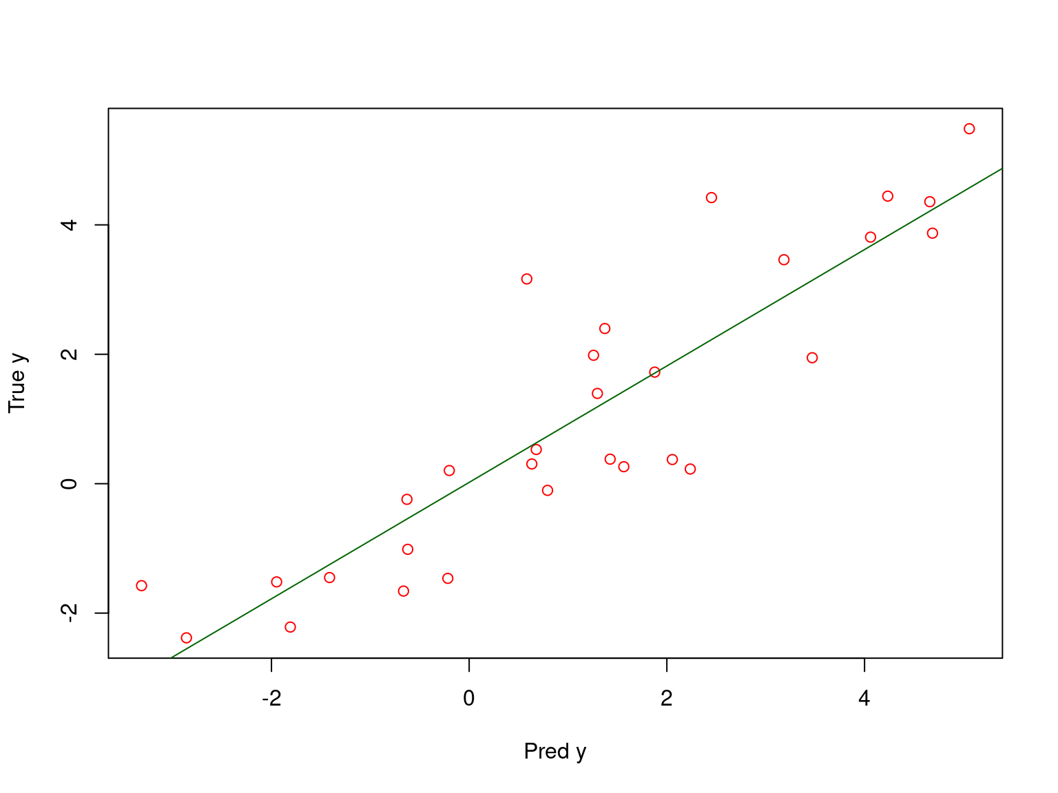
Toy example: model validation
Call:
lm(formula = test$y ~ test_predicted)

Residuals:
     Min       1Q   Median       3Q      Max
-1.80597 -0.78005  0.07636  0.52330  2.61924

Coefficients:
               Estimate Std. Error t value Pr(>|t|)
(Intercept)     0.02058    0.21588   0.095    0.925
test_predicted  0.89953    0.08678  10.366 4.33e-11 ***
---
Signif. codes:  0 '***' 0.001 '**' 0.01 '*' 0.05 '.' 0.1 ' ' 1

Residual standard error: 1.053 on 28 degrees of freedom
Multiple R-squared:  0.7933,    Adjusted R-squared:  0.7859
F-statistic: 107.4 on 1 and 28 DF,  p-value: 4.329e-11
Thus the model explains 79% of variation on the test subset.
From linear models to artificial neural networks (ANNs)
- ANN: a mathematical function Y = f(X) with a special architecture
- Can be non-linear depending on activation function
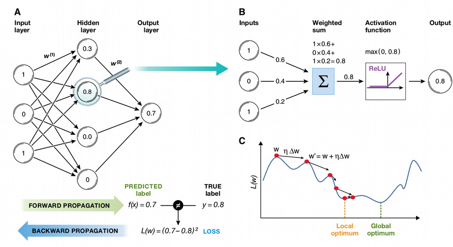
- Backward propagation (gradient descent) for minimizing error
- Universal Approximation Theorem
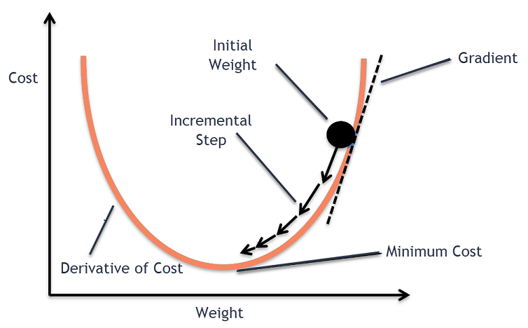
Gradient descent
\[y_i = \alpha + \beta x_i + \epsilon, \,\, i = 1 \ldots n\]
\[E(\alpha, \beta) = \frac{1}{n}\sum_{i=1}^n(y_i - \alpha - \beta x_i)^2\]
\[\hat{\alpha}, \hat{\beta} = \rm{argmin} \,\, E(\alpha, \beta)\]
\[\frac{\partial E(\alpha, \beta)}{\partial\alpha} = -\frac{2}{n}\sum_{i=1}^n(y_i - \alpha - \beta x_i)\]
\[\frac{\partial E(\alpha, \beta)}{\partial\beta} = -\frac{2}{n}\sum_{i=1}^n x_i(y_i - \alpha - \beta x_i)\]
Numeric implementation of gradient descent:
\[\alpha_{i+1} = \alpha_i - \eta \left. \frac{\partial E(\alpha, \beta)}{\partial\alpha} \right\vert_{\alpha=\alpha_i,\beta=\beta_i}\]
\[\beta_{i+1} = \beta_i - \eta \left. \frac{\partial E(\alpha, \beta)}{\partial\beta} \right\vert_{\alpha=\alpha_i,\beta=\beta_i}\]
Coding gradient descent from scratch in R
n <- 100 # sample size
x <- rnorm(n) # simulated expanatory variable
y <- 3 + 2 * x + rnorm(n) # simulated response variable
summary(lm(y ~ x))
Call:
lm(formula = y ~ x)

Residuals:
    Min      1Q  Median      3Q     Max
-1.9073 -0.6835 -0.0875  0.5806  3.2904

Coefficients:
            Estimate Std. Error t value Pr(>|t|)
(Intercept)  2.89720    0.09755   29.70   <2e-16 ***
x            1.94753    0.10688   18.22   <2e-16 ***
---
Signif. codes:  0 '***' 0.001 '**' 0.01 '*' 0.05 '.' 0.1 ' ' 1

Residual standard error: 0.9707 on 98 degrees of freedom
Multiple R-squared:  0.7721,    Adjusted R-squared:  0.7698
F-statistic:   332 on 1 and 98 DF,  p-value: < 2.2e-16
Let us now reconstruct the intercept and slope from gradient descent
alpha <- vector(); beta <- vector()
E <- vector(); dEdalpha <- vector(); dEdbeta <- vector()
eta <- 0.01; alpha[1] <- 1; beta[1] <- 1 # initialize alpha and beta
for(i in 1:1000)
{
  E[i] <- (1/n) * sum((y - alpha[i] - beta[i] * x)^2)
  dEdalpha[i] <- - sum(2 * (y - alpha[i] - beta[i] * x)) / n
  dEdbeta[i] <- - sum(2 * x * (y - alpha[i] - beta[i] * x)) / n

  alpha[i+1] <- alpha[i] - eta * dEdalpha[i]
  beta[i+1] <- beta[i] - eta * dEdbeta[i]
}
print(paste0("alpha = ", tail(alpha, 1),", beta = ", tail(beta, 1)))
[1] "alpha = 2.89719694937354, beta = 1.94752837381973"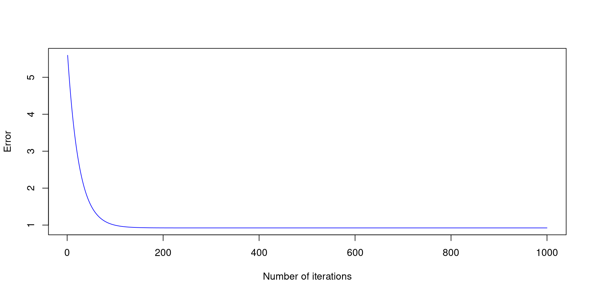
ANN from scratch in R: problem formulation
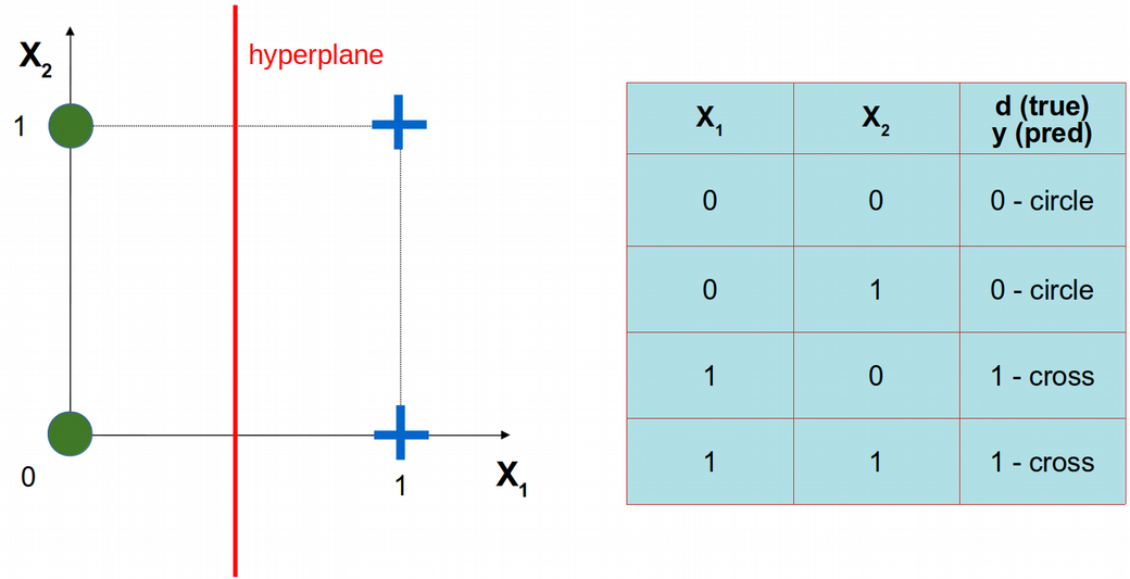
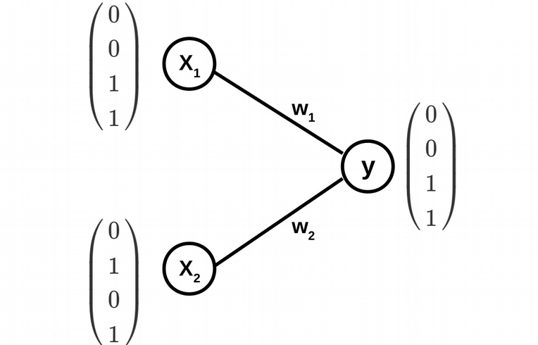
\[y(w_1,w_2)=\phi(w_1x_1+w_2x_2)\]
\[\phi(s)=\frac{1}{1+e^{\displaystyle -s}} \,\,\rm{-}\,\rm{sigmoid}\]
\[\phi^\prime(s)=\phi(s)\left(1-\phi(s)\right)\]
ANN from scratch in R: implementation in code
phi <- function(x){return(1/(1 + exp(-x)))} # activation function

mu <- 0.1; N_epochs <- 10000
w1 <- 0.1; w2 <- 0.5; E <- vector()
for(epochs in 1:N_epochs)
{
  #Forward propagation
  y <- phi(w1 * x1 + w2 * x2 - 3) # we use a fixed bias -3

  #Backward propagation
  E[epochs] <- (1 / (2 * length(d))) * sum((d - y)^2)
  dE_dw1 <- - (1 / length(d)) * sum((d - y) * y * (1 - y) * x1)
  dE_dw2 <- - (1 / length(d)) * sum((d - y) * y * (1 - y) * x2)
  w1 <- w1 - mu * dE_dw1
  w2 <- w2 - mu * dE_dw2
}
plot(E ~ seq(1:N_epochs), xlab="Epochs", ylab="Error", col="red")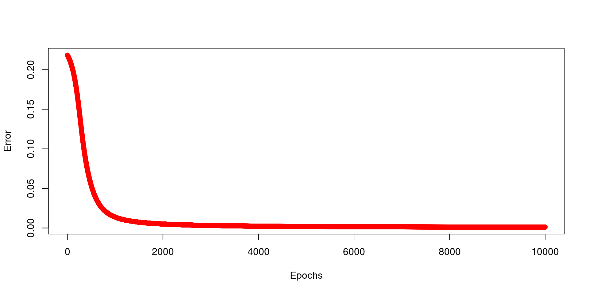
\[E(w_1,w_2)=\frac{1}{2N}\sum_{i=1}^N\left(d_i-y_i(w_1,w_2)\right)^2\]
\[w_{1,2}=w_{1,2}-\mu\frac{\partial E(w_1,w_2)}{\partial w_{1,2}}\]
\[\frac{\partial E}{\partial w_1} = -\frac{1}{N}\sum_{i=1}^N (d_i-y_i)*y_i*(1-y_i)*x_{1i}\]
\[\frac{\partial E}{\partial w_2} = -\frac{1}{N}\sum_{i=1}^N (d_i-y_i)*y_i*(1-y_i)*x_{2i}\]
Decision tree from scratch in R: problem formulation
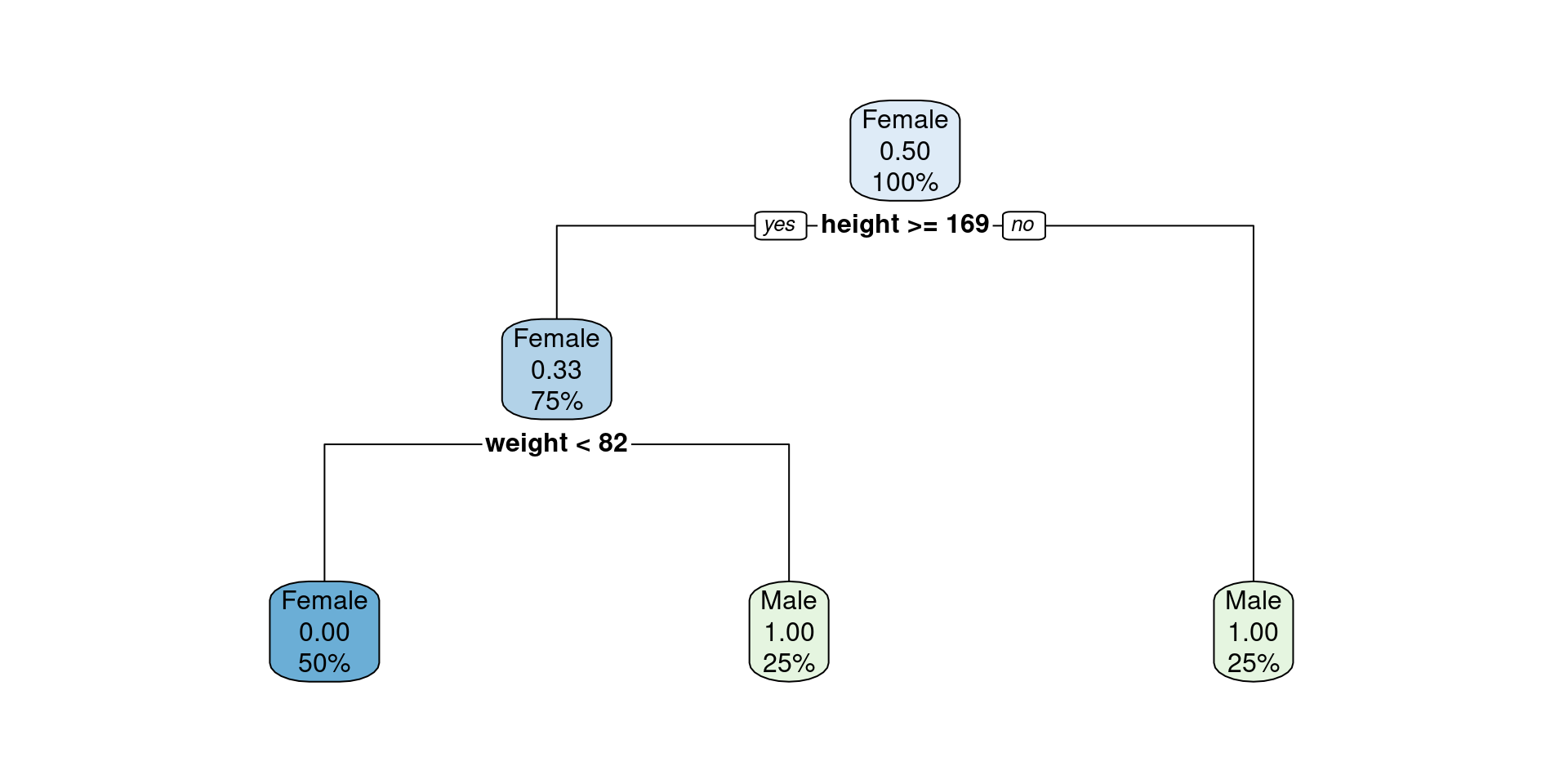
Decision tree from scratch in R: Gini index and split
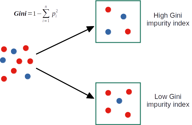
get_best_split <- function(X, y)
{
  mean_gini <- vector(); spl_vals <- vector(); spl_names <- vector()
  for(j in colnames(X)) # for each variable in X data frame
  {
    spl <- vector() # vector of potential split candidates
    sort_X <- X[order(X[, j]), ]; sort_y <- y[order(X[, j])] # sort by variable
    for(i in 1:(dim(X)[1]-1)) # for each observation of variable in X data frame
    {
      spl[i] <- (sort_X[i, j] + sort_X[(i + 1), j]) / 2 # variable consecutive means
      g1_y <- sort_y[sort_X[, j] > spl[i]] # take labels for group above split
      g2_y <- sort_y[sort_X[, j] < spl[i]] # take labels for group below split
      mean_gini <- append(mean_gini, (gini(g1_y) + gini(g2_y))/2) # two groups mean Gini
      spl_vals <- append(spl_vals, spl[i])
      spl_names <- append(spl_names, j)
    }
  }
  min_spl_val <- spl_vals[mean_gini == min(mean_gini)][1] # get best split variable
  min_spl_name <- spl_names[mean_gini == min(mean_gini)][1] # get best split value
  sort_X <- X[order(X[, min_spl_name]), ] # sort X by best split variable
  sort_y <- y[order(X[, min_spl_name])] # sort y by best split variable
  g1_y <- sort_y[sort_X[, min_spl_name] > min_spl_val] # labels above best split
  g2_y <- sort_y[sort_X[, min_spl_name] < min_spl_val] # labels below best split
  if(gini(g1_y) == 0){sex <- paste0("Above: ", as.character(g1_y))}
  else if(gini(g2_y) == 0){sex <- paste0("Below: ", as.character(g2_y))}

  return(list(spl_name = min_spl_name, spl_value = min_spl_val, sex = sex))
}
get_best_split(X, y)
$spl_name
[1] "height"
$spl_value
[1] 169
$sex
[1] "Below: Male"Decision tree from scratch in R: prediction
- Finally, after we have trained the decision tree, we can try to make predictions, and check whether we can reconstruct the labels of the data points
predict_decision_tree <- function(X, y)
{
# Train a decision tree
t <- decision_tree(X, y, max_depth = 2)
# Parse the output of decision tree and code it via if, else if and else
pred_labs <- vector()
for(i in 1:dim(X)[1])
{
if(eval(parse(text=paste0(X[i,t$spl_name[1]],t$sign[1],t$spl_val[1]))))
{
pred_labs[i] <- t$label[1]
}
else if(eval(parse(text=paste0(X[i,t$spl_name[2]],t$sign[2],t$spl_val[2]))))
{
pred_labs[i] <- t$label[2]
}
else{pred_labs[i] <- ifelse(t$label[2] == "Male", "Female", "Male")}
}
return(cbind(cbind(X, y), pred_labs))
}
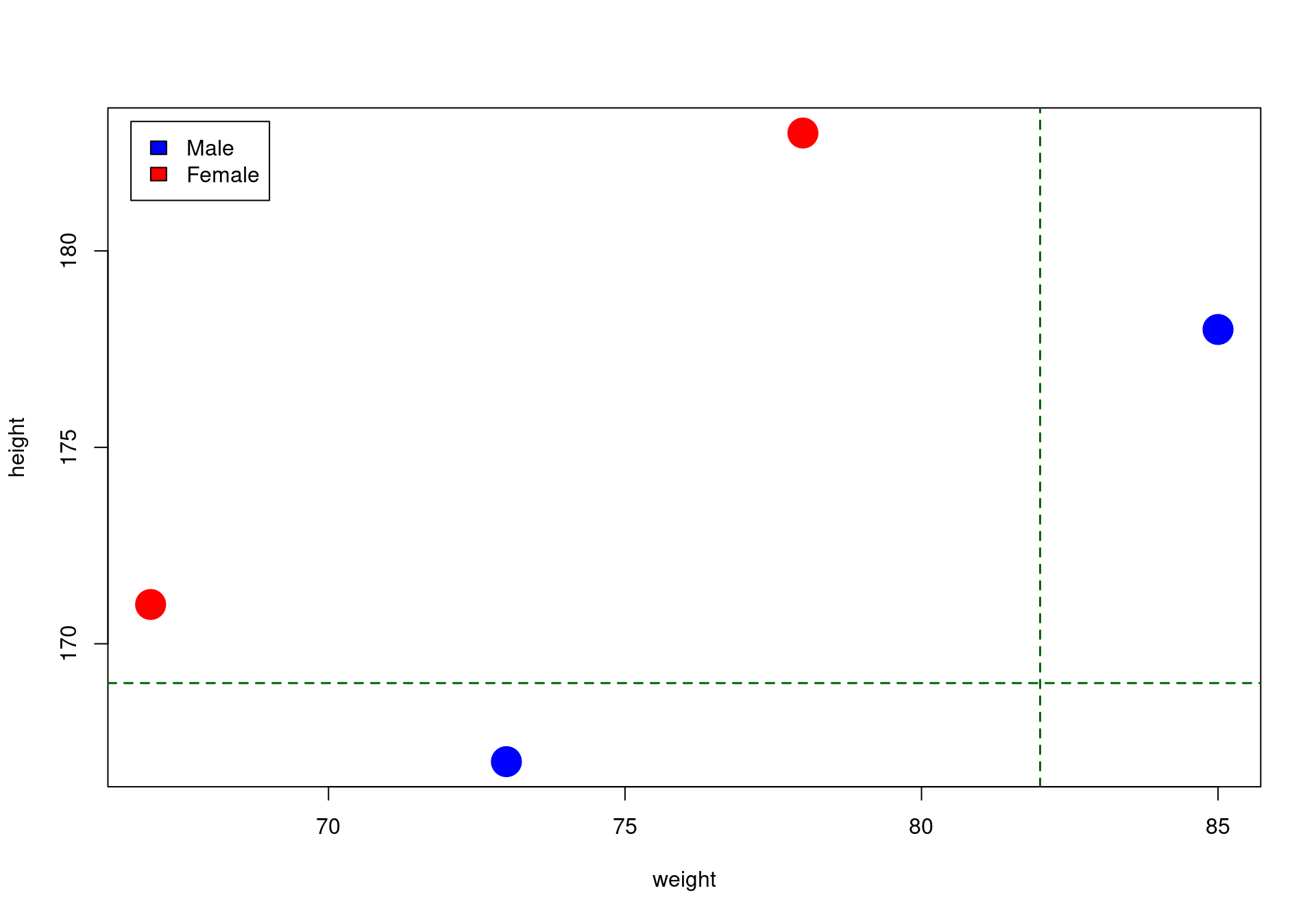
predict_decision_tree(X, y)[1] "All terminal nodes have perfect purity"| height | weight | y | pred_labs |
|---|---|---|---|
| 183 | 78 | Female | Female |
| 167 | 73 | Male | Male |
| 178 | 85 | Male | Male |
| 171 | 67 | Female | Female |
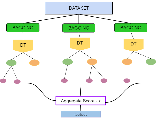
Random Forest has two key differences:
train multiple decision trees (bagging)
train trees on fractions of input features
Thank you! Questions?
         _
platform x86_64-pc-linux-gnu
os       linux-gnu
major    4
minor    3.2
2024 • SciLifeLab • NBIS • RaukR

