Debugging, Profiling, and Optimization

RaukR 2023 • Advanced R for Bioinformatics

Marcin Kierczak

27-Jun-2023

Run Forrest, run!

My code does not run! – debugging
Now it does run but… out of memory! – profiling
It runs! It says it will finish in 5 ~~minutes~~ years. – optimization

Types of bugs

🔣 Syntax errors

prin(var1) 
mean(sum(seq((x + 2) * (y - 9 * b)))

🔢 Arithmetic

y <- 7 / 0

Not in R though! y = Inf

🍎🍊 Type

mean('a')

🧩 Logic

Everything works and produces seemingly valid output that is WRONG!
IMHO those are the hardest 💀 to debug!

How to avoid bugs

Encapsulate your code in smaller units 🍱 (functions), you can test.
Use classes and type checking 🆗.
Test 🧪 at the boundaries, e.g. loops at min and max value.
Feed your functions with test data 💾 that should result with a known output.
Use antibugging 🕸: stopifnot(y <= 75)

Floating confusion

(vec <- seq(0.1, 0.9, by=0.1))
vec == 0.7 
vec == 0.5

[1] 0.1 0.2 0.3 0.4 0.5 0.6 0.7 0.8 0.9
[1] FALSE FALSE FALSE FALSE FALSE FALSE FALSE FALSE FALSE
[1] FALSE FALSE FALSE FALSE  TRUE FALSE FALSE FALSE FALSE

(0.5 + 0.1) - 0.6
(0.7 + 0.1) - 0.8

[1] 0
[1] -1.110223e-16

💀 Beware of floating point arithmetic! 💀

How to float 🏊

round((0.7 + 0.1) , digits = 2) - 0.8

[1] 0

Comparing floating point numbers:

(vec <- seq(0.1, 0.9, by=0.1))
vec == 0.7

[1] 0.1 0.2 0.3 0.4 0.5 0.6 0.7 0.8 0.9
[1] FALSE FALSE FALSE FALSE FALSE FALSE FALSE FALSE FALSE

epsilon <- 0.001
abs(vec - 0.7) <= epsilon

[1] FALSE FALSE FALSE FALSE FALSE FALSE  TRUE FALSE FALSE

Final thoughts on floating

head(unlist(.Machine))

    double.eps double.neg.eps    double.xmin    double.xmax    double.base 
  2.220446e-16   1.110223e-16  2.225074e-308  1.797693e+308   2.000000e+00 
 double.digits 
  5.300000e+01

head(unlist(.Platform))

   OS.type   file.sep dynlib.ext        GUI     endian    pkgType 
    "unix"        "/"   ".dylib"  "unknown"   "little"   "source"

Handling Errors

Let us generate some errors:

input <- c(1, 10, -7, -2/5, 0, 'char', 100, pi, NaN)
for (val in input) {
  (paste0('Log of ', val, 'is ', log10(val)))
}

Error in log10(val): non-numeric argument to mathematical function

So, how to handle this mess?

Handling Errors – `try`

try(
  print(
    paste0('Log of ', input, ' is ', log10(as.numeric(input)))
  )
)

[1] "Log of 1 is 0"                               
[2] "Log of 10 is 1"                              
[3] "Log of -7 is NaN"                            
[4] "Log of -0.4 is NaN"                          
[5] "Log of 0 is -Inf"                            
[6] "Log of char is NA"                           
[7] "Log of 100 is 2"                             
[8] "Log of 3.14159265358979 is 0.497149872694133"
[9] "Log of NaN is NaN"

Handling Errors – `tryCatch` block:

result <- tryCatch(log10(val), 
            warning = function(w) { 
              print('Warning! Negative argument supplied. Negating.') 
              log10(-val) }, 
            error = function(e) { 
              print('ERROR! Not a number!')
              NaN
            }
          )

[1] "Log of 1 is 0"
[1] "Log of 10 is 1"
[1] "Warning! Negative argument supplied. Negating."
[1] "Log of -7 is 0.845098040014257"
[1] "Warning! Negative argument supplied. Negating."
[1] "Log of -0.4 is -0.397940008672038"
[1] "Log of 0 is -Inf"
[1] "Log of NA is NA"
[1] "Log of 100 is 2"
[1] "Log of 3.14159265358979 is 0.497149872694133"
[1] "Log of NaN is NaN"

Debugging – errors and warnings

An error in your code will result in a call to the stop() function that:
- Breaks the execution of the program (loop, if-statement, etc.)
- Performs the action defined by the global parameter error.
A warning just prints out the warning message (or reports it in another way)

Global parameter error defines what R should do when an error occurs.

options(error = )

You can use simpleError() and simpleWarning() to generate errors and warnings in your code:

f <- function(x) {
  if (x < 0) {
    x <- abs(x)
    w <- simpleWarning("Value less than 0. Taking abs(x)")
    w
  }
}

Debugging – what are my options?

Old-school debugging: a lot of print statements
- print values of your variables at some checkpoints,
- sometimes fine but often laborious,
- need to remove/comment out manually after debugging.

Dumping frames
- on error, R state will be saved to a file,
- file can be read into debugger,
- values of all variables can be checked,
- can debug on another machine, e.g. send dump to your colleague!

Traceback
- a list of the recent function calls with values of their parameters

Step-by-step debugging
- execute code line by line within the debugger

Option 1: dumping frames

f <- function(x) { sin(x) }
options(error = quote(dump.frames(dumpto = "assets/testdump", to.file = T)))
f('test')
options(error = NULL) # reset the behavior
load('assets/testdump.rda')
# debugger(testdump)

Hint: Last empty line brings you back to the environments menu.

Option 2: traceback

f <- function(x) { 
  log10(x) 
}
g <- function(x) { 
  f(x) 
}
g('test')

Error in log10(x): non-numeric argument to mathematical function

> traceback()
2: f(x) at #2
1: g("test")

traceback() shows what were the function calls and what parameters were passed to them when the error occurred.

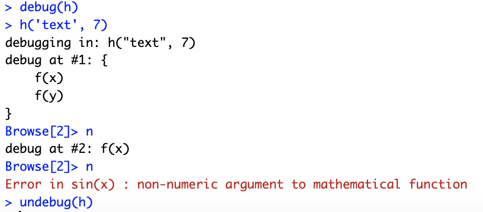
Option 3: step-by-step debugging

Let us define a new function h(x, y):

h <- function(x, y) { 
  f(x) 
  f(y) 
}

Now, we can use debug() to debug the function in a step-by-step manner:

debug(h)
h('text', 7)
undebug(h)

Profiling – `proc.time()`

Profiling is the process of identifying memory and time bottlenecks 🍶 in your code.

proc.time()

   user  system elapsed 
  1.426   0.147   2.113

user time – CPU time charged for the execution of user instructions of the calling process,
system time – CPU time charged for execution by the system on behalf of the calling process,
elapsed time – total CPU time elapsed for the currently running R process.

pt1 <- proc.time()
tmp <- runif(n =  10e5)
pt2 <- proc.time()
pt2 - pt1

   user  system elapsed 
  0.006   0.001   0.007

Profiling – `system.time()`

system.time(runif(n = 10e6))
system.time(rnorm(n = 10e6))

   user  system elapsed 
  0.125   0.006   0.132 
   user  system elapsed 
  0.230   0.005   0.235

An alternative approach is to use tic and toc statements from the tictoc package.

library(tictoc)
tic()
tmp1 <- runif(n = 10e6)
toc()

0.062 sec elapsed

Profiling in action

These 4 functions fill a large vector with values supplied by function f.

1 – loop without memory allocation.

fun_fill_loop1 <- function(n = 10e6, f) {
  result <- NULL
  for (i in 1:n) {
    result <- c(result, eval(call(f, 1)))
  }
  return(result)
}

2 – loop with memory allocation.

fun_fill_loop2 <- function(n = 10e6, f) {
  result <- vector(length = n)
  for (i in 1:n) {
    result[i] <- eval(call(f, 1))
  }
  return(result)
}

Profiling in action cted.

But it is maybe better to use…

vectorization!

3 – vectorized loop without memory allocation.

fun_fill_vec1 <- function(n = 10e6, f) {
  result <- NULL
  result <- eval(call(f, n))
  return(result)
}

4 – vectorized with memory allocation.

fun_fill_vec2 <- function(n = 10e6, f) {
  result <- vector(length = n)
  result <- eval(call(f, n))
  return(result)
}

Profiling our functions

p1 <- system.time(fun_fill_loop1(n = 10e4, "runif")) # 1 - loop, no alloc
p2 <- system.time(fun_fill_loop2(n = 10e4, "runif")) # 2 - loop, alloc 
p3 <- system.time(fun_fill_vec1(n = 10e4, "runif"))  # 3 - vector, no alloc
p4 <- system.time(fun_fill_vec2(n = 10e4, "runif"))  # 4 - vector, alloc

fn	user.self	sys.self	elapsed
fn1	7.007	1.563	8.570
fn2	0.262	0.015	0.276
fn3	0.001	0.000	0.001
fn4	0.001	0.000	0.000

The system.time() function is not the most accurate though. During the lab, we will experiment with package microbenchmark.

More advanced profiling

We can also do a bit more advanced profiling, including the memory profiling, using, e.g. Rprof() function.

Rprof('profiler_test.out', interval = 0.01, memory.profiling = T)
for (i in 1:5) {
  result <- fun_fill_loop2(n = 10e4, "runif")
  print(result)
}
Rprof(NULL)

And let us summarise:

summary <- summaryRprof('profiler_test.out', memory='both')
knitr::kable(summary$by.self)

	self.time	self.pct	total.time	total.pct	mem.total
“print.default”	2.84	59.92	2.84	59.92	2.8
“eval”	0.82	17.30	1.64	34.60	703.2
“runif”	0.63	13.29	0.63	13.29	275.9
“fun_fill_loop2”	0.24	5.06	1.89	39.87	872.6
“parent.frame”	0.08	1.69	0.08	1.69	48.5
“is.list”	0.04	0.84	0.04	0.84	10.5
“is.pairlist”	0.04	0.84	0.04	0.84	0.0
“baseenv”	0.03	0.63	0.03	0.63	6.4
“close.connection”	0.01	0.21	0.01	0.21	0.0
“findCenvVar”	0.01	0.21	0.01	0.21	1.5

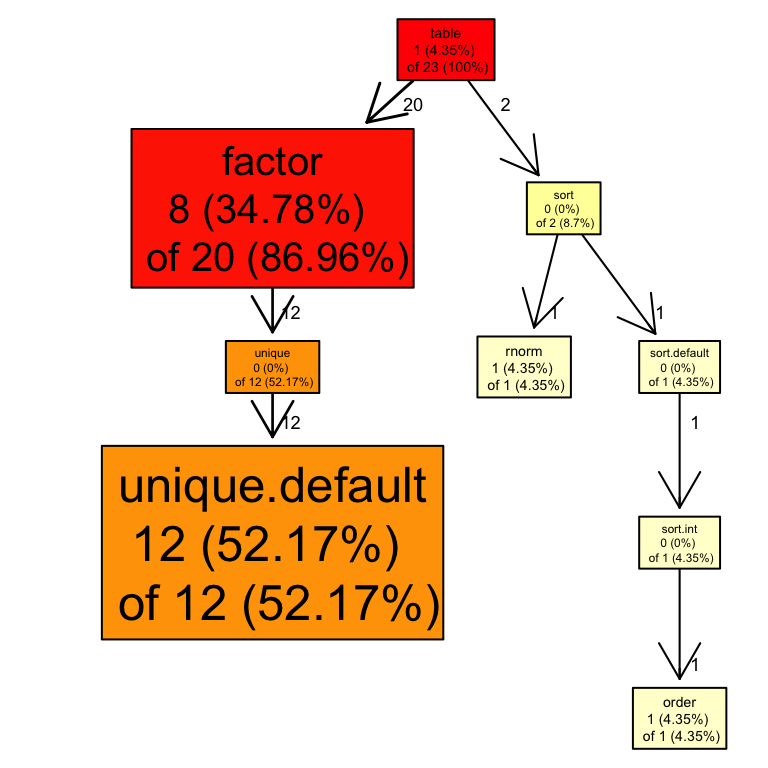
Profiling – `profr` package

There are also packages available that enable even more advanced profiling:

library(profr)
Rprof("profiler_test2.out", interval = 0.01)
tmp <- table(sort(rnorm(1e5)))
Rprof(NULL)
profile_df <- parse_rprof('profiler_test2.out')

This returns a table that can be visualised:

level	g_id	t_id	f	start	end	n	leaf	time	source
1	1	1	table	0.00	0.46	1	FALSE	0.46	base
1	2	1	cb	0.46	0.48	1	FALSE	0.02	NA
2	1	1	sort	0.00	0.04	1	FALSE	0.04	base
2	2	1	factor	0.04	0.46	1	FALSE	0.42	base
2	3	1	tryCatch	0.46	0.48	1	FALSE	0.02	base
3	1	1	rnorm	0.00	0.02	1	TRUE	0.02	stats
3	2	1	sort.default	0.02	0.04	1	FALSE	0.02	base
3	3	1	unique	0.04	0.28	1	FALSE	0.24	base
3	4	2	tryCatchList	0.46	0.48	1	FALSE	0.02	NA
4	1	1	sort.int	0.02	0.04	1	FALSE	0.02	base
4	2	1	unique.default	0.04	0.28	1	TRUE	0.24	base
4	3	2	tryCatchOne	0.46	0.48	1	FALSE	0.02	NA
5	1	1	order	0.02	0.04	1	TRUE	0.02	base
5	2	2	doTryCatch	0.46	0.48	1	FALSE	0.02	NA
6	1	1	inspect_env	0.46	0.48	1	FALSE	0.02	NA
7	1	1	lapply	0.46	0.48	1	FALSE	0.02	base
8	1	1	FUN	0.46	0.48	1	FALSE	0.02	NA
9	1	1	scalar	0.46	0.48	1	FALSE	0.02	NA
10	1	1	trimws	0.46	0.48	1	FALSE	0.02	base
11	1	1	mysub	0.46	0.48	1	FALSE	0.02	NA
12	1	1	sub	0.46	0.48	1	FALSE	0.02	base
13	1	1	is.factor	0.46	0.48	1	FALSE	0.02	base
14	1	1	mysub	0.46	0.48	1	FALSE	0.02	NA
15	1	1	sub	0.46	0.48	1	FALSE	0.02	base
16	1	1	is.factor	0.46	0.48	1	FALSE	0.02	base
17	1	1	try_capture_str	0.46	0.48	1	FALSE	0.02	NA
18	1	1	tryCatch	0.46	0.48	1	FALSE	0.02	base
19	1	1	tryCatchList	0.46	0.48	1	FALSE	0.02	NA
20	1	1	tryCatchOne	0.46	0.48	1	FALSE	0.02	NA
21	1	1	doTryCatch	0.46	0.48	1	FALSE	0.02	NA
22	1	1	capture_str	0.46	0.48	1	FALSE	0.02	NA
23	1	1	paste0	0.46	0.48	1	FALSE	0.02	base
24	1	1	utils::capture.output	0.46	0.48	1	FALSE	0.02	NA
25	1	1	withVisible	0.46	0.48	1	FALSE	0.02	base
26	1	1	…elt	0.46	0.48	1	FALSE	0.02	NA
27	1	1	utils::str	0.46	0.48	1	FALSE	0.02	NA
28	1	1	str.default	0.46	0.48	1	FALSE	0.02	NA
29	1	1	cat	0.46	0.48	1	FALSE	0.02	base
30	1	1	formObj	0.46	0.48	1	FALSE	0.02	NA
31	1	1	maybe_truncate	0.46	0.48	1	FALSE	0.02	NA
32	1	1	nchar.w	0.46	0.48	1	FALSE	0.02	NA
33	1	1	paste	0.46	0.48	1	FALSE	0.02	base
34	1	1	format.fun	0.46	0.48	1	FALSE	0.02	NA
35	1	1	format	0.46	0.48	1	FALSE	0.02	base
36	1	1	format.default	0.46	0.48	1	FALSE	0.02	base
37	1	1	prettyNum	0.46	0.48	1	FALSE	0.02	base
38	1	1	is.na	0.46	0.48	1	TRUE	0.02	base

Profiling – `profr` package cted.

We can also plot the results using – proftools package-

library(Rgraphviz)
library(proftools) # depends on "graph" and "Rgraphviz" packages
profile_df2 <- readProfileData("profiler_test2.out")
plotProfileCallGraph(profile_df2, style = google.style, score = "total")

Profiling with `profvis`

Yet another nice way to profile your code is by using Hadley Wickham’s profvis package:

library(profvis)
profvis({fun_fill_loop2(1e4, 'runif')
  fun_fill_vec2(1e4, 'runif')
})

Profiling with `profvis` cted.

Optimizing your code

We should forget about small efficiencies, say about 97% of the time: premature optimization is the root of all evil. Yet we should not pass up our opportunities in that critical 3%. A good programmer will not be deluded into complacency by such reasoning, he will be wise to look carefully at the critical code; but only after that code has been identified.

– Donald Knuth

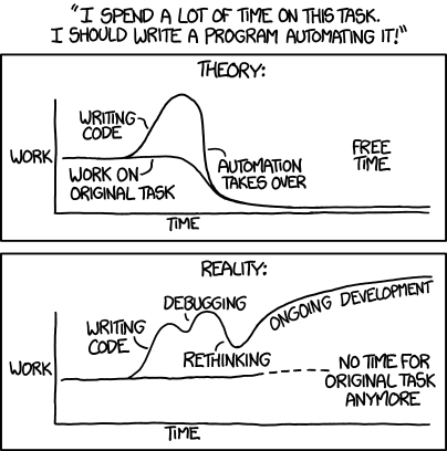
source: http://www.xkcd/com/1319

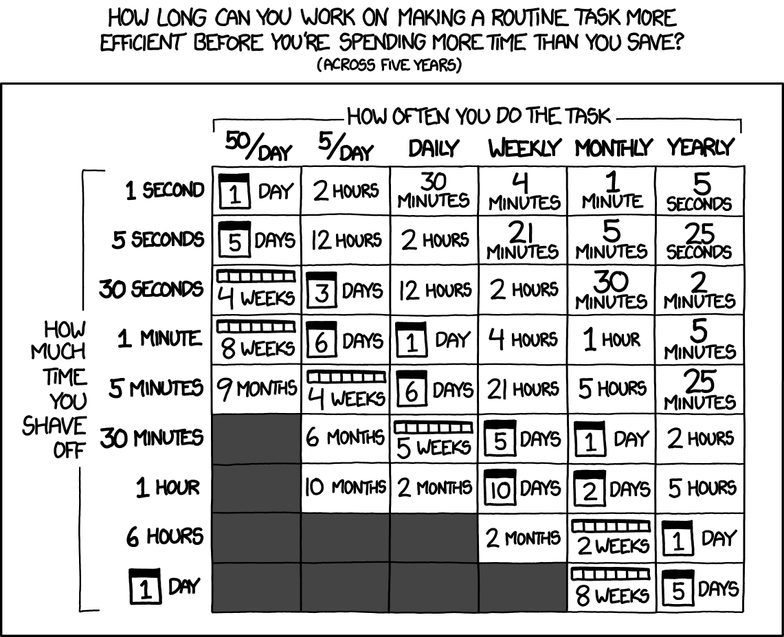
source: http://www.xkcd/com/1205

Ways to optimize the code

write it in a more efficient way, e.g. use vectorization or *apply family instead of loops etc.,
allocating memory to avoid copy-on-modify,
use package BLAS for linear algebra,
use bigmemory package,
GPU computations,
multicore support, e.g. multicore, snow
use futures
use data.table or tibble instead of data.frame

Copy-on-modify

library(pryr)
order <- 1024
matrix_A <- matrix(rnorm(order^2), nrow = order)
matrix_B <- matrix_A

Check where the objects are in the memory:

address(matrix_A)
address(matrix_B)

[1] "0x118000000"
[1] "0x118000000"

What happens if we modify a value in one of the matrices?

matrix_B[1,1] <- 1
address(matrix_A)
address(matrix_B)

[1] "0x118000000"
[1] "0x118804000"

Avoid copying by allocating memory

No memory allocation

f1 <- function(to = 3, silent=F) {
  tmp <- c()
  for (i in 1:to) {
    a1 <- address(tmp)
    tmp <- c(tmp, i)
    a2 <- address(tmp)
    if (!silent) { print(paste0(a1, " --> ", a2)) } 
  }
}
f1()

[1] "0x15a80f4e0 --> 0x13aab2158"
[1] "0x13aab2158 --> 0x13aaa05c8"
[1] "0x13aaa05c8 --> 0x159317708"

Avoid copying by allocating memory cted.

With memory allocation

f2 <- function(to = 3, silent = FALSE) {
  tmp <- vector(length = to, mode='numeric')
  for (i in 1:to) {
    a1 <- address(tmp)
    tmp[i] <- i
    a2 <- address(tmp)
    if(!silent) { print(paste0(a1, " --> ", a2)) }
  }
}
f2()

[1] "0x129363bb8 --> 0x129363bb8"
[1] "0x129363bb8 --> 0x129363bb8"
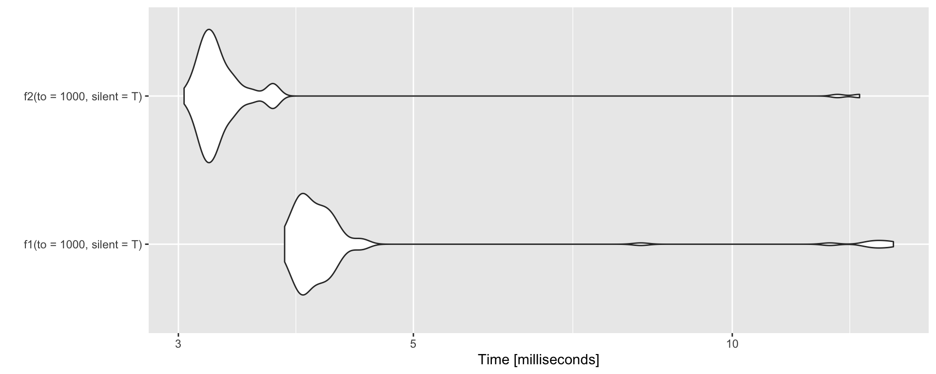
[1] "0x129363bb8 --> 0x129363bb8"

Allocating memory – benchmark.

library(microbenchmark)
benchmrk <- microbenchmark(f1(to = 1e3, silent = T), 
                           f2(to = 1e3, silent = T), 
                           times = 100L)
ggplot2::autoplot(benchmrk)

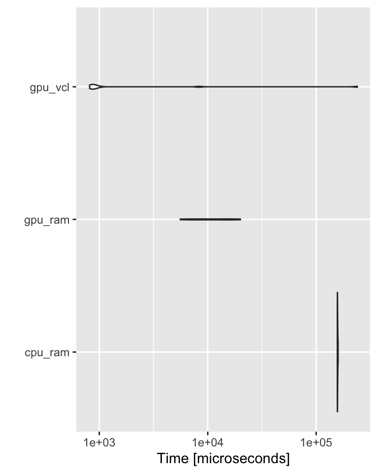
GPU

A = matrix(rnorm(1000^2), nrow=1000) # stored: RAM, computed: CPU
B = matrix(rnorm(1000^2), nrow=1000) 
gpuA = gpuMatrix(A, type = "float") # stored: RAM, computed: GPU
gpuB = gpuMatrix(B, type = "float")
vclA = vclMatrix(A, type = "float") # stored: GPU, computed: GPU
vclB = vclMatrix(B, type = "float")
bch <- microbenchmark(
  cpu_ram = A %*% B,
  gpu_ram = gpuA %*% gpuB,
  gpu_vcl = vclA %*% vclB, 
  times = 10L)

GPU cted.

ggplot2::autoplot(bch)

Parallelization using package `parallel`

Easiest to parallelize is lapply:

result <- lapply(1:2, function(x) { c(x, x^2, x^3) })
result

[[1]]
[1] 1 1 1

[[2]]
[1] 2 4 8

library(parallel)
num_cores <- detectCores() - 1
cl <- makeCluster(num_cores) # Init cluster
parLapply(cl, 1:2, function(x) { c(x, x^2, x^3)} )
stopCluster(cl)

[[1]]
[1] 1 1 1

[[2]]
[1] 2 4 8

Thank you! Questions?

         _                         
platform aarch64-apple-darwin20.0.0
os       darwin20.0.0              
major    4                         
minor    2.2

2023 • SciLifeLab • NBIS • RaukR