Web apps with Shiny

Note

This is an introduction to shiny web applications with R. Please follow the exercise to familiarise yourself with the fundamentals. And then you can follow instructions to build one of the two complete apps.

• Code chunks starting with shinyApp() can be simply copy-pasted to the RStudio console and run.
• Generally, complete shiny code is saved as a text file, named for example, as app.R and then clicking Run app launches the app.

1 UI • Layout

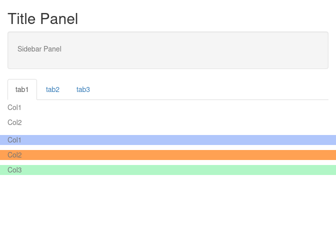
This is an example to show the layout of widgets on a webpage using shiny functions. fluidPage() is used to define a responsive webpage. titlePanel() is used to define the top bar. sidebarLayout() is used to create a layout that includes a region on the left called side bar panel and a main panel on the right. The contents of these panels are further defined under sidebarPanel() and mainPanel().

In the main panel, the use of tab panels are demonstrated. The function tabsetPanel() is used to define a tab panel set and individual tabs are defined using tabPanel(). fluidRow() and column() are used to structure elements within each tab. The width of each column is specified. Total width of columns must add up to 12.

library(shiny)
ui <- fluidPage(
  titlePanel("Title Panel"),
  sidebarLayout(
    sidebarPanel(
      helpText("Sidebar Panel")
    ),
    mainPanel(tabsetPanel(
      tabPanel("tab1",
               fluidRow(
                 column(6,helpText("Col1")),
                 column(6,
                        helpText("Col2"),
                        fluidRow(
                          column(4,style="background-color:#b0c6fb",
                                 helpText("Col1")
                          ),
                          column(4,style="background-color:#ffa153",
                                 helpText("Col2")
                          ),
                          column(4,style="background-color:#b1f6c6",
                                 helpText("Col3")
                          )
                        )
                 )
               )
      ),
      tabPanel("tab2",
               inputPanel(helpText("Input Panel"))
      ),
      tabPanel("tab3",
               wellPanel(helpText("Well Panel"))
      )
    )
    )
  )
)

server <- function(input,output){}
shinyApp(ui=ui,server=server)

2 UI • Widgets • Input

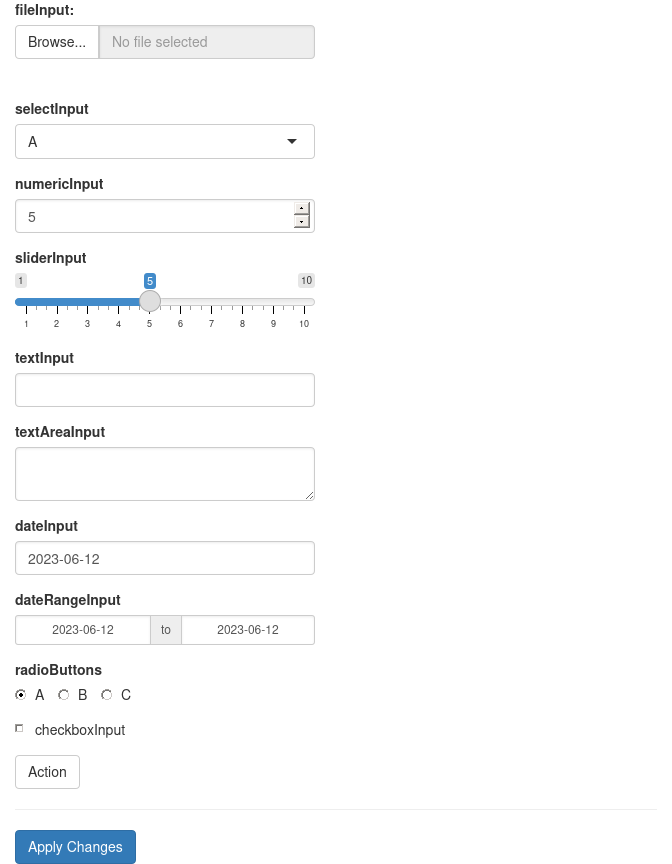
Input widgets are used to accept content interactively from the user. These widgets usually end in Input like selectInput(). Below are usage examples of several of shiny’s built-in widgets. Every widget has a variable name which is accessible through input$ in the server function. For example, the value of a variable named text-input would be accessed through input$text-input.

shinyApp(
ui=fluidPage(
  fluidRow(
    column(6,
           fileInput("file-input","fileInput:"),
           selectInput("select-input",label="selectInput",choices=c("A","B","C")),
           numericInput("numeric-input",label="numericInput",value=5,min=1,max=10),
           sliderInput("slider-input",label="sliderInput",value=5,min=1,max=10),
           textInput("text-input",label="textInput"),
           textAreaInput("text-area-input",label="textAreaInput"),
           dateInput("date-input",label="dateInput"),
           dateRangeInput("date-range-input",label="dateRangeInput"),
           radioButtons("radio-button",label="radioButtons",choices=c("A","B","C"),inline=T),
           checkboxInput("checkbox","checkboxInput",value=FALSE),
           actionButton("action-button","Action"),
           hr(),
           submitButton()
    )
  )
),
server=function(input,output){},
options=list(height=900))

3 UI • Widgets • Outputs

Similar to input widgets, output widgets are used to display information to the user on the webpage. These widgets usually end in Output like textOutput(). Every widget has a variable name accessible under output$ to which content is written in the server function. Render functions are used to write content to output widgets. For example renderText() is used to write text data to textOutput() widget.

shinyApp(
  ui=fluidPage(fluidRow(column(6,
             textInput("text_input",label="textInput",value="<h3 style='color:red'>Red text</h3>"),
             hr(),
             htmlOutput("html_output"),
             textOutput("text_output"),
             verbatimTextOutput("verbatim_text_output"),
             tableOutput("table_output"),
             plotOutput("plot_output",width="300px",height="300px")
      ))),
  server=function(input, output) {
    output$html_output <- renderText({input$text_input})
    output$text_output <- renderText({input$text_input})
    output$verbatim_text_output <- renderText({input$text_input})
    output$table_output <- renderTable({iris[1:3,1:3]})
    output$plot_output <- renderPlot({
      plot(iris[,1],iris[,2])
    })
},
options=list(height=700))

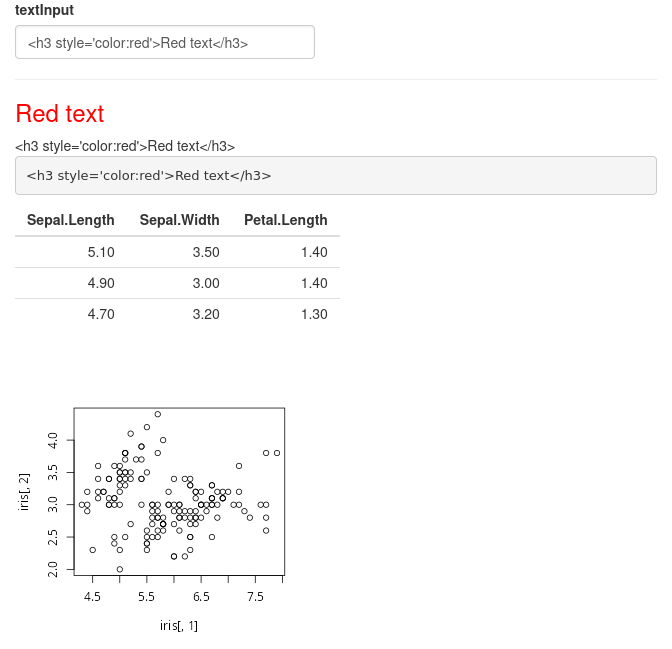
In this example, we have a text input box which takes user text and outputs it in three different variations. The first output is html output htmlOutput(). Since the default text is html content, the output is red colored text. A normal non-html text would just look like normal text. The second output is normal text output textOutput(). The third variation is verbatimTextOutput() which displays text in monospaced code style. This example further shows table output and plot output.

4 Dynamic UI

Sometimes we want to add, remove or change currently loaded UI widgets conditionally based on dynamic changes in code execution or user input. Conditional UI can be defined using conditionalPanel(), uiOutput()/renderUI(), insertUI() or removeUI. In this example, we will use uiOutput()/renderUI().

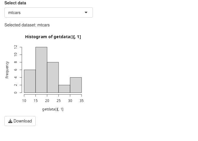
In the example below, the output plot is displayed only if the selected dataset is iris.

shinyApp(
ui=fluidPage(
  selectInput("data_input",label="Select data",
              choices=c("mtcars","faithful","iris")),
  tableOutput("table_output"),
  uiOutput("ui")
),

server=function(input,output) {
  getdata <- reactive({ get(input$data_input, 'package:datasets') })
  
  output$ui <- renderUI({
    if(input$data_input=="iris") plotOutput("plot_output",width="400px")
  })
  
  output$plot_output <- renderPlot({hist(getdata()[, 1])})
  output$table_output <- renderTable({head(getdata())})
})

Here, conditional UI is used to selectively display an output widget (plot). Similarly, this idea can be used to selectively display any input or output widget.

5 Updating widgets

Widgets can be updated with new values dynamically. observe() and observeEvent() functions can monitor the values of interest and update relevant widgets.

shinyApp(
ui=fluidPage(
  selectInput("data_input",label="Select data",choices=c("mtcars","faithful","iris")),
  selectInput("header_input",label="Select column name",choices=NULL),
  plotOutput("plot_output",width="400px")
),

server=function(input,output,session) {
  getdata <- reactive({ get(input$data_input, 'package:datasets') })
  
  observe({
    updateSelectInput(session,"header_input",label="Select column name",choices=colnames(getdata()))
  })
  
  output$plot_output <- renderPlot({
    #shiny::req(input$header_input)
    #validate(need(input$header_input %in% colnames(getdata()),message="Incorrect column name."))
    hist(getdata()[, input$header_input],xlab=input$header_input,main=input$data_input)
  })
},
options=list(height=600))

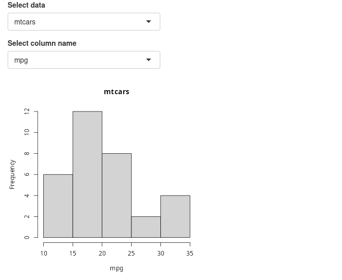
In this example, the user selects a dataset and a column from the selected dataset to be plotted as a histogram. The column name selection widget must automatically update it’s choices depending on the selected dataset. This achieved using observe() where the updateSelectInput() function updates the selection choices. Notice that a third option session is in use in the server function. ie; server=function(input,output,session). And session is also the first argument in updateSelectInput(). Session keeps track of values in the current session.

When changing the datasets, we can see that there is a short red error message. This is because, after we have selected a new dataset, the old column name from the previous dataset is searched for in the new dataset. This occurs for a short time and causes the error. This can be fixed using careful error handling. We will discuss this in another section.

6 Isolate

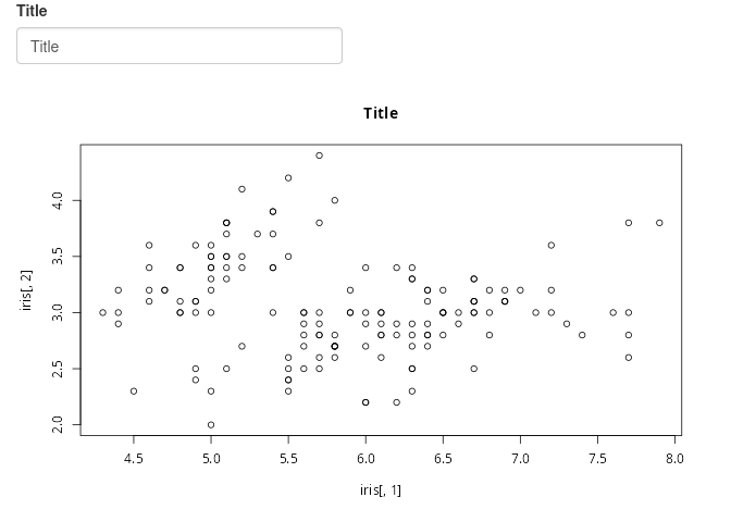
You might’ve noticed that shiny tends to update changes immediately as the input widgets change. This may not be desirable in all circumstances. For example, if the apps runs a heavy calculation, it is more efficient to grab all the changes and execute in one step rather than executing the heavy calculation after every input change. To illustrate this, we have an example below where we plot an image which has the title as input text. Try adding a long title to it.

shinyApp(
  ui=fluidPage(
    textInput("in_title",label="Title",value="Title"),
    plotOutput("out_plot")),
  
  server=function(input,output) {
    output$out_plot <- renderPlot({
      plot(iris[,1],iris[,2],main=input$in_title)
    })
  }
)

The plot changes as soon as the input text field is changed. And as we type in text, the image is continuously being redrawn. This can be computationally intensive depending on the situation. A better solution would be to write the text completely without any reactivity and when done, let the app know that you are ready to redraw.

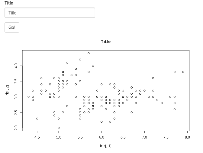
We can add an action button such that the plot is changed only when the button is clicked.

shinyApp(
  ui=fluidPage(
    textInput("in_title",label="Title",value="Title"),
    actionButton("btn_go","Go!"),
    plotOutput("out_plot")),
  
  server=function(input,output) {
    output$out_plot <- renderPlot({
      input$btn_go
      plot(iris[,1],iris[,2],main=isolate(input$in_title))
    })
  }
)

Now, changes to any of the input fields do not initiate the plot function. The plot is redrawn only when the action button is clicked. When the action button is click, the current values in the input fields are collected and used in the plotting function.

7 Error validation

Shiny returns an error when a variable is NULL, NA or empty. This is similar to normal R operation. The errors show up as bright red text. By using careful error handling, we can print more informative and less distracting error messages. We also have the option of hiding error messages.

shinyApp(
ui=fluidPage(
  selectInput("data_input",label="Select data",
              choices=c("","mtcars","faithful","iris")),
  tableOutput("table_output")
),

server=function(input, output) {
  getdata <- reactive({ get(input$data_input,'package:datasets') })
  output$table_output <- renderTable({head(getdata())})
},
options=list(height="350px"))

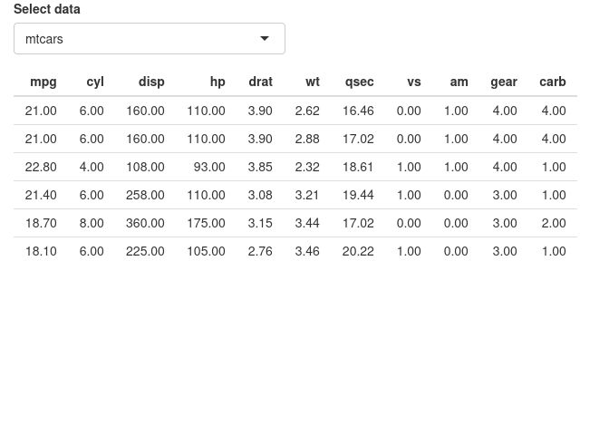
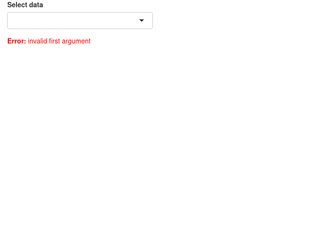
In this example, we have a list of datasets to select which is then printed as a table. The first and default option is an empty string which cannot be printed as a table and therefore returns an error.

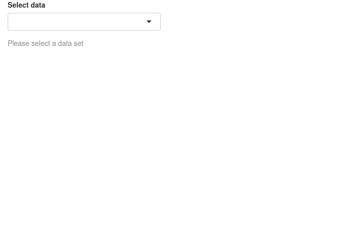
We can add an extra line to the above app so that the selected string is validated before running downstream commands in the getdata({}) reactive function. The function validate() is used to validate inputs. validate() can be used with need() function or a custom function.

Below we use the need() function to check the input. It checks if the input is NULL, NA or an empty string and returns a specified message if TRUE. try() is optional and is used to catch any other unexpected errors.

shinyApp(
ui=fluidPage(
  selectInput("data_input",label="Select data",
              choices=c("","mtcars","faithful","iris")),
  tableOutput("table_output")
),

server=function(input, output) {
  
  getdata <- reactive({
    validate(need(try(input$data_input),"Please select a data set"))
    get(input$data_input,'package:datasets')
  })
  
  output$table_output <- renderTable({head(getdata())})
},
options=list(height="350px"))

Now we see an informative gray message (less scary) asking the user to select a dataset.

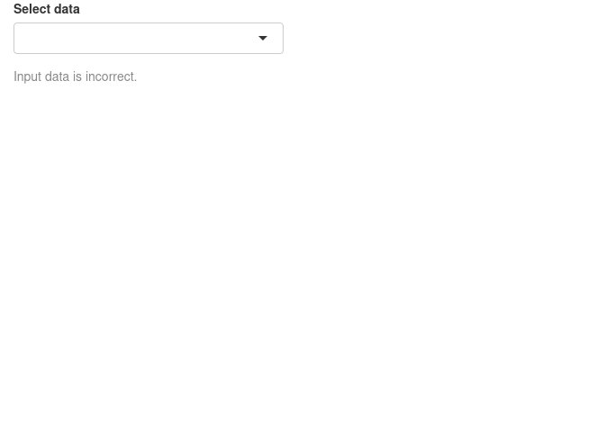
We can use a custom function instead of using need(). Below, we have created a function called valfun() that checks if the input is NULL, NA or an empty string. This is then used in validate().

valfn <- function(x) if(is.null(x) | is.na(x) | x=="") return("Input data is incorrect.")

shinyApp(
ui=fluidPage(
  selectInput("data_input",label="Select data",
              choices=c("","mtcars","faithful","iris")),
  tableOutput("table_output")
),

server=function(input, output) {
  
  getdata <- reactive({
    validate(valfn(try(input$data_input)))
    get(input$data_input,'package:datasets')
  })
  
  output$table_output <- renderTable({head(getdata())})
},
options=list(height="350px"))

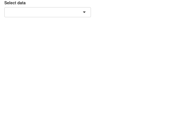
The last option is to simple hide the error. This may be used in situations where there is no input needed from the user. We use req() to check if the input is valid, else stop execution there till the condition becomes true.

shinyApp(
ui=fluidPage(
  selectInput("data_input",label="Select data",
              choices=c("","mtcars","faithful","iris")),
  tableOutput("table_output")
),

server=function(input, output) {
  
  getdata <- reactive({
    shiny::req(try(input$data_input))
    get(input$data_input,'package:datasets')
  })
  
  output$table_output <- renderTable({head(getdata())})
},
options=list(height="350px"))

As expected there is no error or any message at all. This is not always the best to use this option as we need the user to do something. An informative message may be better than nothing.

Finally, instead of printing messages about the error or hiding the error, we can try to resolve the errors from the previous section in a more robust manner. shiny::req(input$header_input) is added to ensure that a valid column name string is available before running any of the renderPlot() commands. Second, we add validate(need(input$header_input %in% colnames(getdata()),message="Incorrect column name.")) to ensure that the column name is actually a column in the currently selected dataset.

shinyApp(
ui=fluidPage(
  selectInput("data_input",label="Select data",choices=c("mtcars","faithful","iris")),
  selectInput("header_input",label="Select column name",choices=NULL),
  plotOutput("plot_output",width="400px")
),

server=function(input,output,session) {
  getdata <- reactive({ get(input$data_input, 'package:datasets') })
  
  observe({
    updateSelectInput(session,"header_input",label="Select column name",choices=colnames(getdata()))
  })
  
  output$plot_output <- renderPlot({
    shiny::req(input$header_input)
    validate(need(input$header_input %in% colnames(getdata()),message="Incorrect column name."))
    hist(getdata()[, input$header_input],xlab=input$header_input,main=input$data_input)
  })
},
options=list(height=600))

Now, we do not see any error messages. Note that shiny apps on shinyapps.io do not display the complete regular R error message for security reasons. It returns a generic error message in the app. One needs to inspect the error logs to view the actual error message.

8 Download • Data

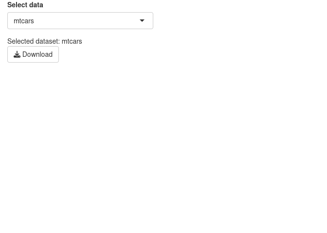
It is often desirable to let the user down data tables and plots as images. This is done using downloadHandler().

In the example below, we are downloading a table as a csv text file. We define a button that accepts the action input from the user. The downloadHandler() function has the file name argument, and the content argument where we specify the write.csv() command. Note that this example needs to be opened in a browser and may not in the RStudio preview. In the RStudio preview, click on Open in Browser.

shinyApp(
  ui=fluidPage(
    selectInput("data_input",label="Select data",
                choices=c("mtcars","faithful","iris")),
    textOutput("text_output"),
    downloadButton("button_download","Download")
  ),

  server=function(input, output) {
    
    getdata <- reactive({ get(input$data_input, 'package:datasets') })
    output$text_output <- renderText(paste0("Selected dataset: ",input$data_input))
    
    output$button_download <- downloadHandler(
      filename = function() {
        paste0(input$data_input,".csv")
      },
      content = function(file) {
        write.csv(getdata(),file,row.names=FALSE,quote=F)
      })
  },
  options=list(height="200px")
)

9 Download • Plot

In this next example, we are downloading a plot. In the content part of downloadHandler(), we specify commands to export a PNG image. Note that this example needs to be opened in a browser and may not in the RStudio preview. In the RStudio preview, click on Open in Browser.

shinyApp(
  ui=fluidPage(
    selectInput("data_input",label="Select data",
                choices=c("mtcars","faithful","iris")),
    textOutput("text_output"),
    plotOutput("plot_output",height="300px",width="300px"),
    downloadButton("button_download","Download")
  ),

  server=function(input, output) {
    
    getdata <- reactive({ get(input$data_input, 'package:datasets') })
    output$text_output <- renderText(paste0("Selected dataset: ",input$data_input))
    
    output$plot_output <- renderPlot({hist(getdata()[,1])})
  
  output$button_download <- downloadHandler(
    filename = function() {
      paste0(input$data_input,".png")
    },
    content = function(file) {
      png(file)
      hist(getdata()[, 1])
      dev.off()
    })
  },
  options=list(height="500px")
)

10 Interactive documents

10.1 Shiny in Rmarkdown

Shiny interactive widgets can be embedded into Rmarkdown documents. These documents need to be live and can handle interactivity. The important addition is the line runtime: shiny to the YAML matter. Here is an example:

---
runtime: shiny
output: html_document
---

```{r}
library(shiny)
```

This is a standard RMarkdown document. Here is some code:

```{r}
head(iris)
```

```{r}
plot(iris$Sepal.Length,iris$Petal.Width)
```

But, here is an interactive shiny widget.

```{r}
sliderInput("in_breaks",label="Breaks:",min=5,max=50,value=5,step=5)
```

```{r}
renderPlot({{
hist(iris$Sepal.Length,breaks=input$in_breaks)
}})
```

This code can be copied to a new file in RStudio and saved as, for example, shiny.Rmd. Then click ‘Knit’. Alternatively, you can run rmarkdown::run("shiny.Rmd").

10.2 Shiny in Quarto

Shiny widgets can be embedded into quarto documents. The YAML needs to specify server: shiny which runs shiny server in the background.

---
title: "This is a title"
format: html
server: shiny
---

```{r}
sliderInput("bins", "Number of bins:", 
            min = 1, max = 50, value = 30)
plotOutput("distPlot")
```

```{r}
#| context: server
output$distPlot <- renderPlot({
  x <- faithful[, 2]  # Old Faithful Geyser data
  bins <- seq(min(x), max(x), length.out = input$bins + 1)
  hist(x, breaks = bins, col = 'darkgray', border = 'white')
})
```

It is also possible to run individual chunks in shiny using context chunk parameter.

```{r}
#| context: server
```

More information about using shiny and quarto together is here.

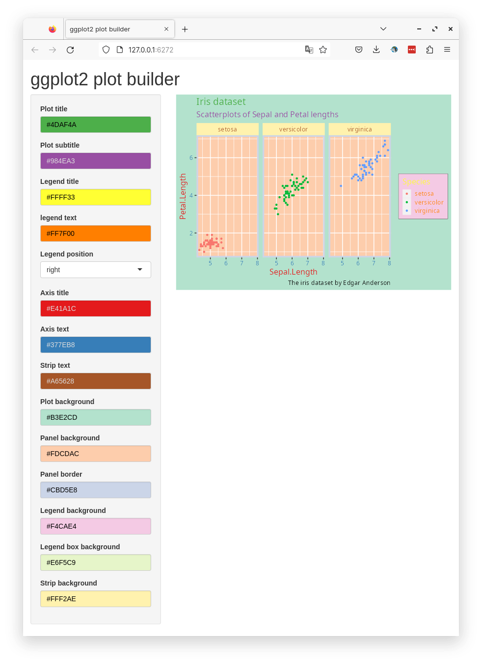
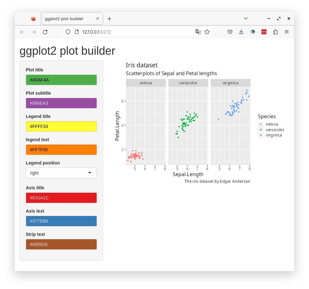
11 ggplot2 builder

In the ggplot2 presentation, we had a few slides with theme customisation. We will try to recreate that as a shiny app, so we can interactively customise a plot.

Topics covered

• UI sidebar layout
• Input and output widgets
• Using colorpicker widget
• Creating plots in a shiny app

The following R packages will be required for this app: ggplot2, shiny, colourpicker.

Below is a preview of the complete app.

We start with a shiny app template with sidebar layout.

library(shiny)

shinyApp(
  ui=pageWithSidebar(
    sidebarPanel(),
    mainPanel()
  ),
  server=function(input,output){
  }
)

In the ui part, we will define inputs. Most of the inputs are colours, so we use the colorInput() widget from the R package colorpicker. The output plot is defined as plotOutput("plot"). In the server part, we define a renderPlot() function that generates a ggplot object.

Code

library(shiny)
library(ggplot2)
library(colourpicker)

shinyApp(
    ui = pageWithSidebar(
        headerPanel("ggplot2 plot builder"),
        sidebarPanel(
            colourInput("in_plot_title", "Plot title", value = "#4daf4a"),
            colourInput("in_plot_subtitle", "Plot subtitle", value = "#984ea3"),
            colourInput("in_legend_title", "Legend title", value = "#ffff33"),
            colourInput("in_legend_text", "legend text", value = "#ff7f00"),
            selectInput("in_legend_pos", "Legend position", choices = c("right", "left", "top", "bottom"), selected = "right"),
            colourInput("in_axis_title", "Axis title", value = "#e41a1c"),
            colourInput("in_axis_text", "Axis text", value = "#377eb8"),
            colourInput("in_strip_text", "Strip text", value = "#a65628"),
        ),
        mainPanel(
            plotOutput("plot")
        )
    ),
    server = function(input, output) {

        output$plot <- renderPlot({
            ggplot(iris, aes(Sepal.Length, Petal.Length, col = Species)) +
                geom_point() +
                facet_wrap(~Species) +
                labs(title = "Iris dataset", subtitle = "Scatterplots of Sepal and Petal lengths", caption = "The iris dataset by Edgar Anderson") +
                theme_grey(base_size = 16)
        })

    }
)

The input widgets now need to be connected to the ggplot function.

Code

library(shiny)
library(ggplot2)
library(colourpicker)

shinyApp(
    ui = pageWithSidebar(
        headerPanel("ggplot2 plot builder"),
        sidebarPanel(
            colourInput("in_plot_title", "Plot title", value = "#4daf4a"),
            colourInput("in_plot_subtitle", "Plot subtitle", value = "#984ea3"),
            colourInput("in_legend_title", "Legend title", value = "#ffff33"),
            colourInput("in_legend_text", "legend text", value = "#ff7f00"),
            selectInput("in_legend_pos", "Legend position", choices = c("right", "left", "top", "bottom"), selected = "right"),
            colourInput("in_axis_title", "Axis title", value = "#e41a1c"),
            colourInput("in_axis_text", "Axis text", value = "#377eb8"),
            colourInput("in_strip_text", "Strip text", value = "#a65628"),
        ),
        mainPanel(
            plotOutput("plot")
        )
    ),
    server = function(input, output) {

        output$plot <- renderPlot({
            ggplot(iris, aes(Sepal.Length, Petal.Length, col = Species)) +
                geom_point() +
                facet_wrap(~Species) +
                labs(title = "Iris dataset", subtitle = "Scatterplots of Sepal and Petal lengths", caption = "The iris dataset by Edgar Anderson") +
                theme_grey(base_size = 16)+
                theme(
                  plot.title=element_text(color=input$in_plot_title),
                  plot.subtitle=element_text(color=input$in_plot_subtitle),
                  legend.title=element_text(color=input$in_legend_title),
                  legend.text=element_text(color=input$in_legend_text),
                  legend.position=input$in_legend_pos,
                  axis.title=element_text(color=input$in_axis_title),
                  axis.text=element_text(color=input$in_axis_text),
                  strip.text=element_text(color=input$in_strip_text)
                )
        })

    }
)

Now try changing the colours of plot elements and hopefully, it should change.

You can add more options to the input if you like, for example; rectangular elements such as backgrounds.

Code

library(shiny)
library(ggplot2)
library(colourpicker)

shinyApp(
    ui = pageWithSidebar(
        headerPanel("ggplot2 plot builder"),
        sidebarPanel(
            colourInput("in_plot_title", "Plot title", value = "#4daf4a"),
            colourInput("in_plot_subtitle", "Plot subtitle", value = "#984ea3"),
            colourInput("in_legend_title", "Legend title", value = "#ffff33"),
            colourInput("in_legend_text", "legend text", value = "#ff7f00"),
            selectInput("in_legend_pos", "Legend position", choices = c("right", "left", "top", "bottom"), selected = "right"),
            colourInput("in_axis_title", "Axis title", value = "#e41a1c"),
            colourInput("in_axis_text", "Axis text", value = "#377eb8"),
            colourInput("in_strip_text", "Strip text", value = "#a65628"),
            colourInput("in_plot_background", "Plot background", value = "#b3e2cd"),
            colourInput("in_panel_background", "Panel background", value = "#fdcdac"),
            colourInput("in_panel_border", "Panel border", value = "#cbd5e8"),
            colourInput("in_legend_background", "Legend background", value = "#f4cae4"),
            colourInput("in_legend_box_background", "Legend box background", value = "#e6f5c9"),
            colourInput("in_strip_background", "Strip background", value = "#fff2ae")
        ),
        mainPanel(
            plotOutput("plot")
        )
    ),
    server = function(input, output) {
        output$plot <- renderPlot({
            ggplot(iris, aes(Sepal.Length, Petal.Length, col = Species)) +
                geom_point() +
                facet_wrap(~Species) +
                labs(title = "Iris dataset", subtitle = "Scatterplots of Sepal and Petal lengths", caption = "The iris dataset by Edgar Anderson") +
                theme_grey(base_size = 16) +
                theme(
                    plot.title = element_text(color = input$in_plot_title),
                    plot.subtitle = element_text(color = input$in_plot_subtitle),
                    legend.title = element_text(color = input$in_legend_title),
                    legend.text = element_text(color = input$in_legend_text),
                    legend.position = input$in_legend_pos,
                    axis.title = element_text(color = input$in_axis_title),
                    axis.text = element_text(color = input$in_axis_text),
                    strip.text = element_text(color = input$in_strip_text),
                    plot.background = element_rect(fill = input$in_plot_background),
                    panel.background = element_rect(fill = input$in_panel_background),
                    panel.border = element_rect(fill = NA, color = input$in_panel_border, size = 3),
                    legend.background = element_rect(fill = input$in_legend_background),
                    legend.box.background = element_rect(fill = input$in_legend_box_background),
                    strip.background = element_rect(fill = input$in_strip_background)
                )
        })
    }
)

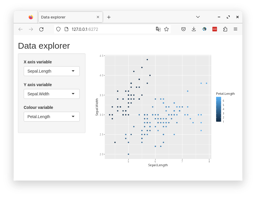
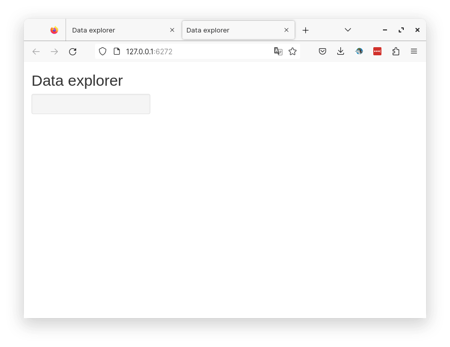
12 Data explorer

A common use case of shiny apps is to explore a dataset interactively. So we will build a simple app that can create a scatterplot from a dataframe which a user can modify interactively. We will use the built-in iris dataset and the user should be able to select x and y axes variables as well the variable mapped to the color of the points.

Topics covered

• UI sidebar layout
• Input and output widgets
• Creating plots in a shiny app
• Passing variables into ggplot through non standard evaluation

The following R packages will be required for this app: ggplot2, shiny.

Below is a preview of the complete app.

12.1 UI

We start with a standard shiny app template.

library(shiny)

shinyApp(
  ui=fluidPage(),
  server=function(input,output){}
)

And then we start building the UI. We will add a title panel and a sidebar layout with a sidebar and a main panel.

library(shiny)

shinyApp(
  ui=fluidPage(
    titlePanel("Data explorer"),
    sidebarLayout(
      sidebarPanel(),
      mainPanel()
    )
  ),
  server=function(input,output){}
)

And to the sidebar, we will add 3 input widgets corresponding to x axis variable, y axis variable and color variable. These will be dropdown type (selectInput()) and choices will be column names of the iris dataframe. And we add the output widget (plotOutput()) in the main panel.

library(shiny)

shinyApp(
  ui=fluidPage(
    titlePanel("Data explorer"),
    sidebarLayout(
      sidebarPanel(
          selectInput("in_x","X axis variable", choices=colnames(iris), selected=colnames(iris)[1], multiple=FALSE),
          selectInput("in_y","Y axis variable", choices=colnames(iris), selected=colnames(iris)[2], multiple=FALSE),
          selectInput("in_col","Colour variable", choices=colnames(iris), selected=colnames(iris)[3], multiple=FALSE)
      ),
      mainPanel(
        plotOutput("out_plot")
      )
    )
  ),
  server=function(input,output){}
)

12.2 Server

Now, we need to add the server part. First, we write the ggplot code to create a plot.

ggplot(iris,aes(x,y,col))+
      geom_point()

This is added inside the output render function renderPlot().

output$out_plot <- renderPlot({
    ggplot(iris,aes(x,y,col))+
      geom_point()
  })

We need to wire the input variable into the ggplot inputs x, y and col. This is achieved through input$ and the variables are wrapped inside !!sym() to convert quoted text to unquoted variable.

output$out_plot <- renderPlot({
  ggplot(iris,aes(!!sym(input$in_x),y=!!sym(input$in_y),col=!!sym(input$in_col)))+
    geom_point()
})

This is finally added to the server function.

You can expand this app to other datasets and map more variables to ggplot etc. Can you add the functionality to download the plots? Or perhaps to upload a csv file and plot from that file?

13 Color generator

A shiny app to create a distinct color generator.

Topics covered

• UI layout using bslib
• Input and output widgets and reactivity
• Use of custom CSS and custom HTML

The following R packages will be required for this app: shiny, hues, bslib.

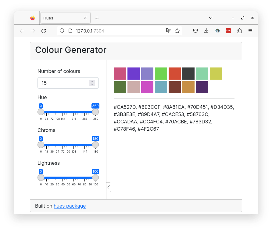
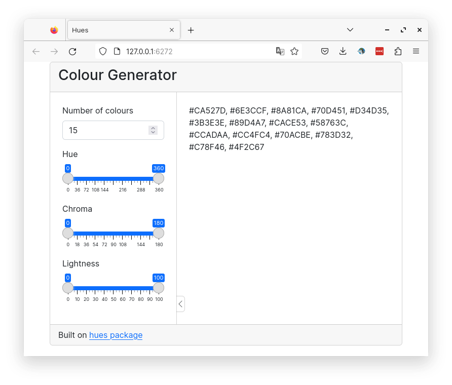
Below is a preview of the finished app.

The core function that generates colors is hues::iwanthue(). What it does is sample colors from the HCL colorspace. Here is an introduction to colorspaces and HCL colorspace. It requires the number of colors to generate.

hues::iwanthue(5)

[1] "#503F44" "#964FB8" "#97B2B7" "#94BF58" "#C6624D"

In addition, this function has six parameters (hmin,hmax,cmin,cmax,lmin,lmax) to control min and max hue, chroma and lightness. This allows you to define where in the HCL colorspace to sample colors from. Hue controls the color wavelength (red, green etc), chroma controls the intensity or saturation of the color and lightness control the brightness.

This gives you mostly warm reddish colors.

hues::iwanthue(5,hmin=0,hmax=5,cmin=80,cmax=160,lmin=38,lmax=70)

[1] "#B82E53" "#D22455" "#D34B6A" "#F16281" "#F22A64"

What we are creating is a graphical user interface around this function.

In this example, we will use the bslib package to create a bootstrap 5 themed layout using cards. See bslib for more info. This is the structure of the app with cards defined inside a fixed page. See help page for bslib::card() for more information on cards. We also define the page title.

library(bslib)

shinyApp(
  ui = page_fixed(
    title = "Hues",
    card(
      card_header(),
      layout_sidebar(
        sidebar()
      ),
      card_footer()
    )
  ),
  server = function(input, output) {
  }
)

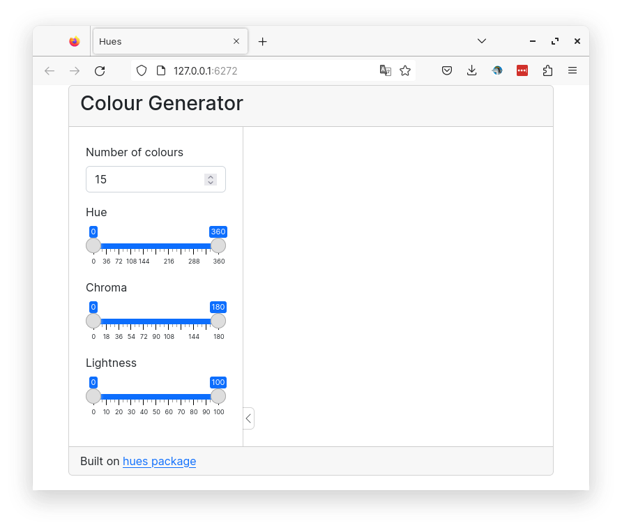
Now we define the inputs in the sidebar panel. The number of colors and the three parameters to the colorspace as ranges. Outside the sidebar panel we define our two outputs: an html output to display the names of the colors as hex values. In the footer, we add an acknowledgement link to the hues package.

library(shiny)
library(hues)
library(bslib)

shinyApp(
  ui = page_fixed(
    title = "Hues",
    card(
      card_header(
        h2("Colour Generator"),
      ),
      layout_sidebar(
        sidebar(
          numericInput("in_n", "Number of colours", value = 15),
          sliderInput("in_hue", "Hue", min = 0, max = 360, value = c(0, 360)),
          sliderInput("in_chr", "Chroma", min = 0, max = 180, value = c(0, 180)),
          sliderInput("in_lig", "Lightness", min = 0, max = 100, value = c(0, 100)),
        ),
        textOutput("out_text")
      ),
      card_footer(
        div("Built on ", a("hues package", href = "https://github.com/johnbaums/hues"))
      )
    )
  ),
  server = function(input, output) {
  }
)

Now, we add content into the server part. The inputs are passed to the get_colours() reactive function. This function is run inside the renderText() function which outputs the colors as hex values.

library(shiny)
library(hues)
library(bslib)

shinyApp(
  ui = page_fixed(
    title = "Hues",
    card(
      card_header(
        h2("Colour Generator"),
      ),
      layout_sidebar(
        sidebar(
          numericInput("in_n", "Number of colours", value = 15),
          sliderInput("in_hue", "Hue", min = 0, max = 360, value = c(0, 360)),
          sliderInput("in_chr", "Chroma", min = 0, max = 180, value = c(0, 180)),
          sliderInput("in_lig", "Lightness", min = 0, max = 100, value = c(0, 100)),
        ),
        textOutput("out_text")
      ),
      card_footer(
        div("Built on ", a("hues package", href = "https://github.com/johnbaums/hues"))
      )
    )
  ),
  server = function(input, output) {
    get_colours <- reactive({
        hues::iwanthue(
            n = input$in_n,
            hmin = min(input$in_hue),
            hmax = max(input$in_hue),
            cmin = min(input$in_chr),
            cmax = max(input$in_chr),
            lmin = min(input$in_lig),
            lmax = max(input$in_lig)
        )
    })

    output$out_text <- renderText({
        cols <- get_colours()
        paste(cols, collapse = ", ")
    })
  }
)

The app will now generate colors as hex values, but we can’t see the colors. It would be nice to visualise the colors. One option would be to create a plot which is generating an image. An alternative lightweight option is to create div elements with the generated colors. For that we add an htmlOutput() element and a new renderText() function to the server part.

This function is creating a span element for each color. These spans are organised inside a div. The div and spans have a parent-child relationship. The span elements are laid out in a grid manner using some custom CSS. The custom CSS is added to the head of the app. We have also added a bit of CSS to add some space above the app so it doesn’t touch the top.

library(shiny)
library(hues)
library(bslib)

shinyApp(
    ui = page_fixed(
      class = "app-container",
      tags$head(tags$style(HTML("
      .app-container {
          margin-top: 1em;
      }

      .grid-parent {
          display: grid;
          gap: 5px;
          grid-template-columns: repeat(auto-fit, minmax(40px, 40px));
      }

      .grid-child {
          height: 40px;
          width: 40px;
      }
    "))),
        title = "Hues",
        card(
            card_header(
                h2("Colour Generator"),
            ),
            layout_sidebar(
                sidebar(
                    numericInput("in_n", "Number of colours", value = 15),
                    sliderInput("in_hue", "Hue", min = 0, max = 360, value = c(0, 360)),
                    sliderInput("in_chr", "Chroma", min = 0, max = 180, value = c(0, 180)),
                    sliderInput("in_lig", "Lightness", min = 0, max = 100, value = c(0, 100)),
                ),
                htmlOutput("out_display"),
                hr(),
                textOutput("out_text")
            ),
            card_footer(
                div("Built on ", a("hues package", href = "https://github.com/johnbaums/hues"))
            )
        )
    ),
    server = function(input, output) {
        get_colours <- reactive({
            hues::iwanthue(
                n = input$in_n,
                hmin = min(input$in_hue),
                hmax = max(input$in_hue),
                cmin = min(input$in_chr),
                cmax = max(input$in_chr),
                lmin = min(input$in_lig),
                lmax = max(input$in_lig)
            )
        })

        output$out_display <- renderText({
            cols <- get_colours()
            paste("<div class='grid-parent'>", paste("<span class='grid-child' style='background-color:", cols, ";'>  </span>", collapse = ""), "</div>", sep = "", collapse = "")
        })

        output$out_text <- renderText({
            cols <- get_colours()
            paste(cols, collapse = ", ")
        })
    }
)

14 RNA-Seq power

Run power analysis for an RNA-Seq experiment.

Topics covered

• UI layout using pre-defined function (pageWithSidebar)
• Input and output widgets and reactivity
• Conditional widgets based on user input
• Validating inputs and custom error messages
• Custom theme

The following R packages are required for this app: c(shiny, shinythemes). In addition, install RNASeqPower from Bioconductor. BiocManager::install('RNASeqPower').

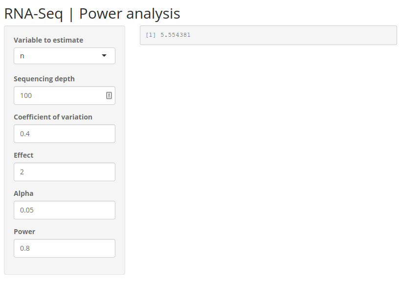
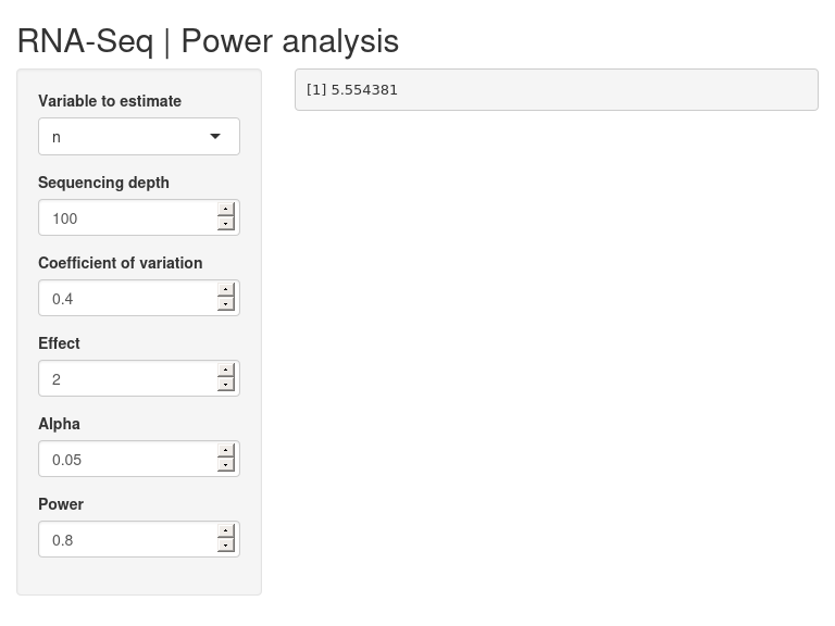
Below is a preview of the complete app.

14.1 RNASeqPower

The R package RNASeqPower helps users to perform a power analysis before running an RNA-Seq experiment. It helps you to estimate, for example, the number of samples required to detect a certain level of significance. The idea of this shiny app is to create a GUI for the RNASeqPower package.

So we first need to understand how RNASeqPower works. For a complete understanding, check out RNASeqPower. For our purpose, we will take a brief look at how it works. We only need to use one function rnapower(). Check out ?RNASeqPower::rnapower.

So, let’s say we want to find out how many samples are required per group. We have some known input parameters. Let’s say the sequencing depth is 50 (depth=50), coefficient of variation is 0.6 (cv=0.6), effect size is 1.5 fold change (effect=1.5), significance cut-off is 0.05 (alpha=0.05) and lastly power of the test is 0.8 (power=0.8). The parameter we want to compute is the number of samples (n), therefore it is not specified.

library(RNASeqPower)
RNASeqPower::rnapower(depth=1000,cv=0.6,effect=2,alpha=0.05,power=0.8)

[1] 11.79489

And we get the number of samples required given these input conditions.

Similarly, we can estimate any of the other parameters (except depth). We can try another example where we solve for power. What would the power be for a study with 12 samples per group, to detect a 2-fold change, given deep (50x) coverage?

rnapower(depth=50, n=12, cv=0.6, effect=2, alpha=.05)

[1] 0.7864965

And the function has returned the power.

Now the idea is to create a web application take these input parameters from the user through input widgets.

14.2 Scaffolding

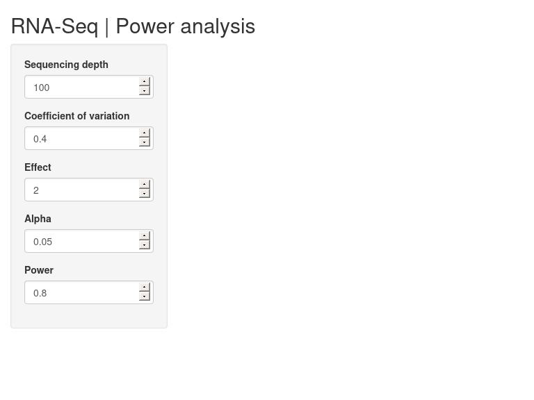
Let’s build the basic scaffolding for our app including the input widgets. Let’s assume we are estimating number of samples.

We use a sidebar layout. The input controls go on the sidebar panel and the output goes on the main panel. So we need 5 numeric inputs. We can set some default values as well as reasonable min and max values and steps to increase or decrease. The output will be verbatim text, so we use verbatimTextOutput() widget.

library(shiny)

shinyApp(
  ui=fluidPage(
    titlePanel("RNA-Seq | Power analysis"),
    sidebarLayout(
      sidebarPanel(
          numericInput("in_pa_depth","Sequencing depth",value=100,min=1,max=1000,step=5),
          numericInput("in_pa_cv","Coefficient of variation",value=0.4,min=0,max=1,step=0.1),
          numericInput("in_pa_effect","Effect",value=2,min=0,max=10,step=0.1),
          numericInput("in_pa_alpha","Alpha",value=0.05,min=0.01,max=0.1,step=0.01),
          numericInput("in_pa_power","Power",value=0.8,min=0,max=1,step=0.1),
      ),
      mainPanel(
        verbatimTextOutput("out_pa")
      )
    )
  ),
  server=function(input,output){
  },
  options=list(height="500px")
)

The app should visually look close to our final end result. Check that the widgets work.

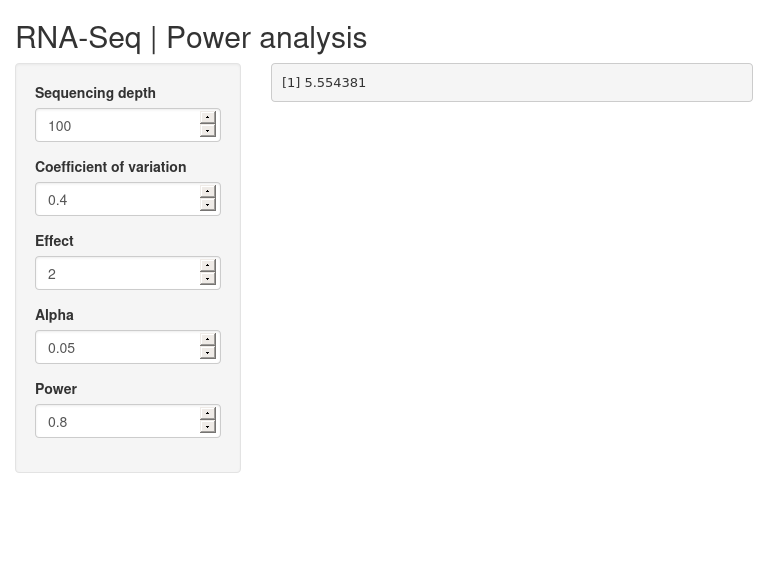
The next step is to wire up the inputs to the rnapower() function and return the result to the output text field.

Try to see if you can get this to work.

library(shiny)
library(RNASeqPower)

shinyApp(
  ui=fluidPage(
    titlePanel("RNA-Seq | Power analysis"),
    sidebarLayout(
      sidebarPanel(
          numericInput("in_pa_depth","Sequencing depth",value=100,min=1,max=1000,step=5),
          numericInput("in_pa_cv","Coefficient of variation",value=0.4,min=0,max=1,step=0.1),
          numericInput("in_pa_effect","Effect",value=2,min=0,max=10,step=0.1),
          numericInput("in_pa_alpha","Alpha",value=0.05,min=0.01,max=0.1,step=0.01),
          numericInput("in_pa_power","Power",value=0.8,min=0,max=1,step=0.1),
      ),
      mainPanel(
        verbatimTextOutput("out_pa")
      )
    )
  ),
  server=function(input,output){
    output$out_pa <- renderPrint({
      rnapower(depth=input$in_pa_depth, cv=input$in_pa_cv, 
               effect=input$in_pa_effect, alpha=input$in_pa_alpha,
               power=input$in_pa_power)
    })
  }
)

Verify that the inputs and outputs work. One can stop at this point if you only need to compute number of samples. But, we will continue to enhance the app to be able to compute any of the other parameters.

14.3 Conditional UI

The function can estimate not only sample size, but cv, effect, alpha or power. We should let the user choose what they want to compute. So, we need a selection input widget to enable selection. And the input fields must change depending on the user’s selected choice. The rnapower() function must also use a different set of parameters depending on the selection choice. For conditional logic, you can chain if else statements or use switch().

Try to add a selection based conditional UI. ?selectInput(), ?uiOutput(), ?renderUI().

library(shiny)
library(RNASeqPower)

shinyApp(
  ui=fluidPage(
    titlePanel("RNA-Seq | Power analysis"),
    sidebarLayout(
      sidebarPanel(
          selectInput("in_pa_est","Variable to estimate",choices=c("n","cv","effect","alpha","power"),selected=1,multiple=FALSE),
          uiOutput("ui_pa")
      ),
      mainPanel(
        verbatimTextOutput("out_pa")
      )
    )
  ),
  server=function(input,output){
    
    output$ui_pa <- renderUI({
      switch(input$in_pa_est,
      "n"=div(
          numericInput("in_pa_depth","Sequencing depth",value=100,min=1,max=1000,step=5),
          numericInput("in_pa_cv","Coefficient of variation",value=0.4,min=0,max=1,step=0.1),
          numericInput("in_pa_effect","Effect",value=2,min=0,max=10,step=0.1),
          numericInput("in_pa_alpha","Alpha",value=0.05,min=0.01,max=0.1,step=0.01),
          numericInput("in_pa_power","Power",value=0.8,min=0,max=1,step=0.1)
        ),
      "cv"=div(
          numericInput("in_pa_depth","Sequencing depth",value=100,min=1,max=1000,step=5),
          numericInput("in_pa_n","Sample size",value=12,min=3,max=1000,step=1),
          numericInput("in_pa_effect","Effect",value=2,min=0,max=10,step=0.1),
          numericInput("in_pa_alpha","Alpha",value=0.05,min=0.01,max=0.1,step=0.01),
          numericInput("in_pa_power","Power",value=0.8,min=0,max=1,step=0.1)
        ),
      "effect"=div(
          numericInput("in_pa_depth","Sequencing depth",value=100,min=1,max=1000,step=5),
          numericInput("in_pa_n","Sample size",value=12,min=3,max=1000,step=1),
          numericInput("in_pa_cv","Coefficient of variation",value=0.4,min=0,max=1,step=0.1),
          numericInput("in_pa_alpha","Alpha",value=0.05,min=0.01,max=0.1,step=0.01),
          numericInput("in_pa_power","Power",value=0.8,min=0,max=1,step=0.1)
        ),
      "alpha"=div(
          numericInput("in_pa_depth","Sequencing depth",value=100,min=1,max=1000,step=5),
          numericInput("in_pa_n","Sample size",value=12,min=3,max=1000,step=1),
          numericInput("in_pa_cv","Coefficient of variation",value=0.4,min=0,max=1,step=0.1),
          numericInput("in_pa_effect","Effect",value=2,min=0,max=10,step=0.1),
          numericInput("in_pa_power","Power",value=0.8,min=0,max=1,step=0.1)
        ),
      "power"=div(
          numericInput("in_pa_depth","Sequencing depth",value=100,min=1,max=1000,step=5),
          numericInput("in_pa_n","Sample size",value=12,min=3,max=1000,step=1),
          numericInput("in_pa_cv","Coefficient of variation",value=0.4,min=0,max=1,step=0.1),
          numericInput("in_pa_effect","Effect",value=2,min=0,max=10,step=0.1),
          numericInput("in_pa_alpha","Alpha",value=0.05,min=0.01,max=0.1,step=0.01)
        )
      )
    })
    
    output$out_pa <- renderPrint({
      
      switch(input$in_pa_est,
        "n"=rnapower(depth=input$in_pa_depth, cv=input$in_pa_cv, 
               effect=input$in_pa_effect, alpha=input$in_pa_alpha,
               power=input$in_pa_power),
        "cv"=rnapower(depth=input$in_pa_depth, n=input$in_pa_n,
               effect=input$in_pa_effect, alpha=input$in_pa_alpha,
               power=input$in_pa_power),
        "effect"=rnapower(depth=input$in_pa_depth, cv=input$in_pa_cv, 
               n=input$in_pa_n, alpha=input$in_pa_alpha,
               power=input$in_pa_power),
        "alpha"=rnapower(depth=input$in_pa_depth, cv=input$in_pa_cv, 
               effect=input$in_pa_effect, n=input$in_pa_n,
               power=input$in_pa_power),
        "power"=rnapower(depth=input$in_pa_depth, cv=input$in_pa_cv, 
               effect=input$in_pa_effect, alpha=input$in_pa_alpha,
               n=input$in_pa_n),
      )
      
    })
  }
)

Let’s summarize what we have done. In the ui part, instead of directly including the rnapower() input variable in the sidebarPanel(), we have added a selection input and a conditional UI output. The content inside the output UI depends on the selection made by the user.

selectInput("in_pa_est", "Variable to estimate", choices=c("n","cv","effect","alpha","power"), selected=1, multiple=FALSE),
uiOutput("ui_pa")

Now to the server part where we make this all work. All conditional UI elements are inside renderUI({}) and we use a conditional logic inside it. And since we are returning multiple input widgets, they are all wrapped inside a div() container.

output$ui_pa <- renderUI({
  switch(input$in_pa_est,
      "n"=div(),
      "cv"=div()
  )
})

In the renderPrint({}) function, we use a similar idea. rnapower() is calculated conditionally based on the user selection.

14.4 Multiple numeric input

Another feature of the rnapower() function that we have not discussed so far is that all the input arguments can take more than one number as input. Or in other words, instead of a single number, it can take a vector of number. For example;

RNASeqPower::rnapower(depth=c(50,100),cv=0.6,effect=1.5,alpha=0.05,power=0.8)

      50      100 
36.28393 35.32909 

And it expands the results in various ways.

RNASeqPower::rnapower(depth=50,cv=0.6,effect=c(1.5,2,3),alpha=0.05,power=0.8)

      1.5         2         3 
36.283928 12.415675  4.942337 

RNASeqPower::rnapower(depth=50,cv=c(0.4,0.6),effect=c(1.5,2,3),alpha=0.05,power=0.8)

         1.5         2        3
0.4 17.18712  5.881109 2.341107
0.6 36.28393 12.415675 4.942337

The output expands in a bit unpredictable manner and this is the reason why our output widget type is set to verbatimTextOutput({}). Otherwise, we could have formatted it to perhaps, a neater table.

How do we incorporate this into our app interface? Ponder over this and try to come up with solutions.

One way to do it is to accept comma separated values from the user. And then parse that into a vector of numbers. For example;

x <- "2.5,6"
as.numeric(unlist(strsplit(gsub(" ","",x),",")))

[1] 2.5 6.0

Blank space are removed, the string is split by comma into a list of strings, the list is converted to a vector and the strings are coerced to numbers.

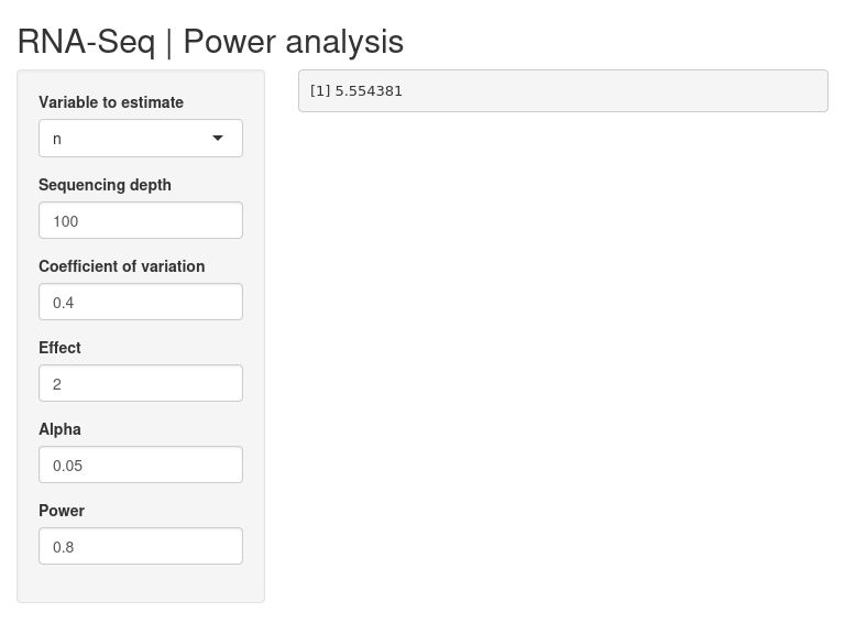
Update the app such that all numeric inputs are replaced by text inputs and the server logic is able to parse the strings into numbers.

library(shiny)
library(RNASeqPower)

shinyApp(
  ui=fluidPage(
    titlePanel("RNA-Seq | Power analysis"),
    sidebarLayout(
      sidebarPanel(
          selectInput("in_pa_est","Variable to estimate",choices=c("n","cv","effect","alpha","power"),selected=1,multiple=FALSE),
          uiOutput("ui_pa")
      ),
      mainPanel(
        verbatimTextOutput("out_pa")
      )
    )
  ),
  server=function(input,output){
    
    output$ui_pa <- renderUI({
      switch(input$in_pa_est,
      "n"=div(
          textInput("in_pa_depth","Sequencing depth",value=100),
          textInput("in_pa_cv","Coefficient of variation",value=0.4),
          textInput("in_pa_effect","Effect",value=2),
          textInput("in_pa_alpha","Alpha",value=0.05),
          textInput("in_pa_power","Power",value=0.8)
        ),
      "cv"=div(
          textInput("in_pa_depth","Sequencing depth",value=100),
          textInput("in_pa_n","Sample size",value=12),
          textInput("in_pa_effect","Effect",value=2),
          textInput("in_pa_alpha","Alpha",value=0.05),
          textInput("in_pa_power","Power",value=0.8)
        ),
      "effect"=div(
          textInput("in_pa_depth","Sequencing depth",value=100),
          textInput("in_pa_n","Sample size",value=12),
          textInput("in_pa_cv","Coefficient of variation",value=0.4),
          textInput("in_pa_alpha","Alpha",value=0.05),
          textInput("in_pa_power","Power",value=0.8)
        ),
      "alpha"=div(
          textInput("in_pa_depth","Sequencing depth",value=100),
          textInput("in_pa_n","Sample size",value=12),
          textInput("in_pa_cv","Coefficient of variation"),
          textInput("in_pa_effect","Effect",value=2),
          textInput("in_pa_power","Power",value=0.8)
        ),
      "power"=div(
          textInput("in_pa_depth","Sequencing depth",value=100),
          textInput("in_pa_n","Sample size",value=12),
          textInput("in_pa_cv","Coefficient of variation",value=0.4),
          textInput("in_pa_effect","Effect",value=2),
          textInput("in_pa_alpha","Alpha",value=0.05)
        )
      )
    })
    
    output$out_pa <- renderPrint({
      
      switch(input$in_pa_est,
        "n"={
          depth <- as.numeric(unlist(strsplit(gsub(" ","",input$in_pa_depth),",")))
          cv <- as.numeric(unlist(strsplit(gsub(" ","",input$in_pa_cv),",")))
          effect <- as.numeric(unlist(strsplit(gsub(" ","",input$in_pa_effect),",")))
          alpha <- as.numeric(unlist(strsplit(gsub(" ","",input$in_pa_alpha),",")))
          power <- as.numeric(unlist(strsplit(gsub(" ","",input$in_pa_power),",")))
          rnapower(depth=depth, cv=cv, effect=effect, alpha=alpha, power=power)
          },
        "cv"={
          depth <- as.numeric(unlist(strsplit(gsub(" ","",input$in_pa_depth),",")))
          n <- as.numeric(unlist(strsplit(gsub(" ","",input$in_pa_n),",")))
          effect <- as.numeric(unlist(strsplit(gsub(" ","",input$in_pa_effect),",")))
          alpha <- as.numeric(unlist(strsplit(gsub(" ","",input$in_pa_alpha),",")))
          power <- as.numeric(unlist(strsplit(gsub(" ","",input$in_pa_power),",")))
          rnapower(depth=depth, n=n, effect=effect, alpha=alpha, power=power)
        },
        "effect"={
          depth <- as.numeric(unlist(strsplit(gsub(" ","",input$in_pa_depth),",")))
          n <- as.numeric(unlist(strsplit(gsub(" ","",input$in_pa_n),",")))
          cv <- as.numeric(unlist(strsplit(gsub(" ","",input$in_pa_cv),",")))
          alpha <- as.numeric(unlist(strsplit(gsub(" ","",input$in_pa_alpha),",")))
          power <- as.numeric(unlist(strsplit(gsub(" ","",input$in_pa_power),",")))
          rnapower(depth=depth, cv=cv, n=n, alpha=alpha, power=power)
        },
        "alpha"={
          depth <- as.numeric(unlist(strsplit(gsub(" ","",input$in_pa_depth),",")))
          n <- as.numeric(unlist(strsplit(gsub(" ","",input$in_pa_n),",")))
          cv <- as.numeric(unlist(strsplit(gsub(" ","",input$in_pa_cv),",")))
          effect <- as.numeric(unlist(strsplit(gsub(" ","",input$in_pa_effect),",")))
          power <- as.numeric(unlist(strsplit(gsub(" ","",input$in_pa_power),",")))
          rnapower(depth=depth, cv=cv, effect=effect, n=n, power=power)
        },
        "power"={
          depth <- as.numeric(unlist(strsplit(gsub(" ","",input$in_pa_depth),",")))
          n <- as.numeric(unlist(strsplit(gsub(" ","",input$in_pa_n),",")))
          cv <- as.numeric(unlist(strsplit(gsub(" ","",input$in_pa_cv),",")))
          effect <- as.numeric(unlist(strsplit(gsub(" ","",input$in_pa_effect),",")))
          alpha <- as.numeric(unlist(strsplit(gsub(" ","",input$in_pa_alpha),",")))
          rnapower(depth=depth, cv=cv, effect=effect, alpha=alpha, n=n)
        },
      )
      
    })
  }
)

To summarize our changes, in the ui part, all numericInput() has been changed to textInput() and in the process we lost the number specific input limits such as min, max, step size etc. In the server part, incoming strings are parsed and split into a vector of numbers, saved to a variable and passed to the rnapower() function. Ensure that the app works without errors and we can progress further.

14.5 Code cleaning

It is good practice to check whether the current code can be cleaned-up/polished or reduced. In this example, depth is always needed and could be moved out of the conditional block. Only one variable changes based on user input, but all 5 variables are repeated in each conditional block. There is room for improvement there.

Try to figure out how the code can be reorganized and simplified.

library(shiny)
library(RNASeqPower)

shinyApp(
  ui=fluidPage(
    titlePanel("RNA-Seq | Power analysis"),
    sidebarLayout(
      sidebarPanel(
          selectInput("in_pa_est","Variable to estimate",choices=c("n","cv","effect","alpha","power"),selected=1,multiple=FALSE),
          uiOutput("ui_pa")
      ),
      mainPanel(
        verbatimTextOutput("out_pa")
      )
    )
  ),
  server=function(input,output){
    
    output$ui_pa <- renderUI({
      div(
        textInput("in_pa_depth","Sequencing depth",value=4),
        if(input$in_pa_est != "n")  textInput("in_pa_n","Sample size",value=100),
        if(input$in_pa_est != "cv")  textInput("in_pa_cv","Coefficient of variation",value=0.4),
        if(input$in_pa_est != "effect")  textInput("in_pa_effect","Effect",value=2),
        if(input$in_pa_est != "alpha")  textInput("in_pa_alpha","Alpha",value=0.05),
        if(input$in_pa_est != "power")  textInput("in_pa_power","Power",value=0.8)
      )
    })
    
    output$out_pa <- renderPrint({
          depth <- as.numeric(unlist(strsplit(gsub(" ","",input$in_pa_depth),",")))
          if(input$in_pa_est != "n")  n <- as.numeric(unlist(strsplit(gsub(" ","",input$in_pa_n),",")))
          if(input$in_pa_est != "cv") cv <- as.numeric(unlist(strsplit(gsub(" ","",input$in_pa_cv),",")))
          if(input$in_pa_est != "effect") effect <- as.numeric(unlist(strsplit(gsub(" ","",input$in_pa_effect),",")))
          if(input$in_pa_est != "alpha")  alpha <- as.numeric(unlist(strsplit(gsub(" ","",input$in_pa_alpha),",")))
          if(input$in_pa_est != "power")  power <- as.numeric(unlist(strsplit(gsub(" ","",input$in_pa_power),",")))
            
      switch(input$in_pa_est,
        "n"=rnapower(depth=depth, cv=cv, effect=effect, alpha=alpha, power=power),
        "cv"=rnapower(depth=depth, n=n, effect=effect, alpha=alpha, power=power),
        "effect"=rnapower(depth=depth, cv=cv, n=n, alpha=alpha, power=power),
        "alpha"=rnapower(depth=depth, cv=cv, effect=effect, n=n, power=power),
        "power"=rnapower(depth=depth, cv=cv, effect=effect, alpha=alpha, n=n)
      )
      
    })
  }
)

UI and server blocks have been considerably reduced in length by removing redundant code.

14.6 Input validation

When we changed numeric inputs to character, we lost the input limits and numeric validation. Regardless of what input you enter, the app tries to proceed with the calculation.

Try entering some unreasonable inputs and see what happens. Try entering random strings, or huge integers for alpha etc.

We can bring back input validation manually using validate() functions. This can be used to check if the input conforms to some expected range of values and if not, return a message to the user.

Here are the limits we want to set:

• depth: A numeric
• n: A numeric
• cv: A numeric
• effect: A numeric
• alpha: A numeric between 0 and 1 excluding 0 and 1
• power: A numeric between 0 and 1 excluding 0 and 1

Try to figure out how to add input validation. ?shiny::validate().

library(shiny)
library(RNASeqPower)

# returns a message if condition is true
fn_validate <- function(input,message) if(input) print(message)

shinyApp(
  ui=fluidPage(
    titlePanel("RNA-Seq | Power analysis"),
    sidebarLayout(
      sidebarPanel(
          selectInput("in_pa_est","Variable to estimate",choices=c("n","cv","effect","alpha","power"),selected=1,multiple=FALSE),
          uiOutput("ui_pa")
      ),
      mainPanel(
        verbatimTextOutput("out_pa")
      )
    )
  ),
  server=function(input,output){
    
    output$ui_pa <- renderUI({
      div(
        textInput("in_pa_depth","Sequencing depth",value=100),
        if(input$in_pa_est != "n")  textInput("in_pa_n","Sample size",value=12),
        if(input$in_pa_est != "cv")  textInput("in_pa_cv","Coefficient of variation",value=0.4),
        if(input$in_pa_est != "effect")  textInput("in_pa_effect","Effect",value=2),
        if(input$in_pa_est != "alpha")  textInput("in_pa_alpha","Alpha",value=0.05),
        if(input$in_pa_est != "power")  textInput("in_pa_power","Power",value=0.8)
      )
    })
    
    output$out_pa <- renderPrint({
          depth <- as.numeric(unlist(strsplit(gsub(" ","",input$in_pa_depth),",")))
          validate(fn_validate(any(is.na(depth)),"Sequencing depth must be a numeric."))
          
          if(input$in_pa_est != "n") {
            n <- as.numeric(unlist(strsplit(gsub(" ","",input$in_pa_n),",")))       
            validate(fn_validate(any(is.na(n)),"Sample size must be a numeric."))
          }
          
          if(input$in_pa_est != "cv") {
            cv <- as.numeric(unlist(strsplit(gsub(" ","",input$in_pa_cv),",")))
            validate(fn_validate(any(is.na(cv)),"Coefficient of variation must be a numeric."))
          }
          
          if(input$in_pa_est != "effect") {
            effect <- as.numeric(unlist(strsplit(gsub(" ","",input$in_pa_effect),",")))
            validate(fn_validate(any(is.na(effect)),"Effect must be a numeric."))
          }
          
          if(input$in_pa_est != "alpha")  {
            alpha <- as.numeric(unlist(strsplit(gsub(" ","",input$in_pa_alpha),",")))
            validate(fn_validate(any(is.na(alpha)),"Alpha must be a numeric."))
            validate(fn_validate(any(alpha>=1|alpha<=0),"Alpha must be a numeric between 0 and 1."))
          }
          
          if(input$in_pa_est != "power")  {
            power <- as.numeric(unlist(strsplit(gsub(" ","",input$in_pa_power),",")))
            validate(fn_validate(any(is.na(power)),"Power must be a numeric."))
            validate(fn_validate(any(power>=1|power<=0),"Power must be a numeric between 0 and 1."))
          }
            
      switch(input$in_pa_est,
        "n"=rnapower(depth=depth, cv=cv, effect=effect, alpha=alpha, power=power),
        "cv"=rnapower(depth=depth, n=n, effect=effect, alpha=alpha, power=power),
        "effect"=rnapower(depth=depth, cv=cv, n=n, alpha=alpha, power=power),
        "alpha"=rnapower(depth=depth, cv=cv, effect=effect, n=n, power=power),
        "power"=rnapower(depth=depth, cv=cv, effect=effect, alpha=alpha, n=n)
      )
      
    })
  }
)

We have added validate() to all incoming text to ensure that user input is within reasonable limits.

Test that the validation works by inputting unreasonable inputs such as alphabets, symbols etc into the input fields.

14.7 Theme

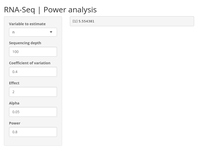
This part is purely cosmetic. We can add a custom theme from R package shinythemes to make our app stand out from the default. The theme is added as an argument to fluidPage() like so fluidPage(theme = shinytheme("spacelab")).

Try changing the theme and pick one that you like. Check out ?shinythemes. The themes can be visualized on Bootswatch.

library(shiny)
library(shinythemes)
library(RNASeqPower)

# returns a message if condition is true
fn_validate <- function(input,message) if(input) print(message)

shinyApp(
  ui=fluidPage(
    theme=shinytheme("spacelab"),
    titlePanel("RNA-Seq | Power analysis"),
    sidebarLayout(
      sidebarPanel(
        selectInput("in_pa_est","Variable to estimate",choices=c("n","cv","effect","alpha","power"),selected=1,multiple=FALSE),
        uiOutput("ui_pa")
      ),
      mainPanel(
        verbatimTextOutput("out_pa")
      )
    )
  ),
  server=function(input,output){
    
    output$ui_pa <- renderUI({
      div(
        textInput("in_pa_depth","Sequencing depth",value=100),
        if(input$in_pa_est != "n")  textInput("in_pa_n","Sample size",value=12),
        if(input$in_pa_est != "cv")  textInput("in_pa_cv","Coefficient of variation",value=0.4),
        if(input$in_pa_est != "effect")  textInput("in_pa_effect","Effect",value=2),
        if(input$in_pa_est != "alpha")  textInput("in_pa_alpha","Alpha",value=0.05),
        if(input$in_pa_est != "power")  textInput("in_pa_power","Power",value=0.8)
      )
    })
    
    output$out_pa <- renderPrint({
      
        depth <- as.numeric(unlist(strsplit(gsub(" ","",input$in_pa_depth),",")))
        validate(fn_validate(any(is.na(depth)),"Sequencing depth must be a numeric."))
        
        if(input$in_pa_est != "n") {
          n <- as.numeric(unlist(strsplit(gsub(" ","",input$in_pa_n),",")))       
          validate(fn_validate(any(is.na(n)),"Sample size must be a numeric."))
        }
        
        if(input$in_pa_est != "cv") {
          cv <- as.numeric(unlist(strsplit(gsub(" ","",input$in_pa_cv),",")))
          validate(fn_validate(any(is.na(cv)),"Coefficient of variation must be a numeric."))
        }
        
        if(input$in_pa_est != "effect") {
          effect <- as.numeric(unlist(strsplit(gsub(" ","",input$in_pa_effect),",")))
          validate(fn_validate(any(is.na(effect)),"Effect must be a numeric."))
        }
        
        if(input$in_pa_est != "alpha")  {
          alpha <- as.numeric(unlist(strsplit(gsub(" ","",input$in_pa_alpha),",")))
          validate(fn_validate(any(is.na(alpha)),"Alpha must be a numeric."))
          validate(fn_validate(any(alpha>=1|alpha<=0),"Alpha must be a numeric between 0 and 1."))
        }
        
        if(input$in_pa_est != "power")  {
          power <- as.numeric(unlist(strsplit(gsub(" ","",input$in_pa_power),",")))
          validate(fn_validate(any(is.na(power)),"Power must be a numeric."))
          validate(fn_validate(any(power>=1|power<=0),"Power must be a numeric between 0 and 1."))
        }
        
        switch(input$in_pa_est,
               "n"=rnapower(depth=depth, cv=cv, effect=effect, alpha=alpha, power=power),
               "cv"=rnapower(depth=depth, n=n, effect=effect, alpha=alpha, power=power),
               "effect"=rnapower(depth=depth, cv=cv, n=n, alpha=alpha, power=power),
               "alpha"=rnapower(depth=depth, cv=cv, effect=effect, n=n, power=power),
               "power"=rnapower(depth=depth, cv=cv, effect=effect, alpha=alpha, n=n)
        )
    })
  }
)

This is the completed app.

14.8 Deployment

You do not necessarily need to do this section. This is just so you know.

The app is now ready to be deployed. If you have an account on shinyapps.io, you can quickly deploy this app to your account using the R package rsconnect.

library(rsconnect)
rsconnect::setAccountInfo(name="username", token="KJHF853HG6G59C2F4J7B6", secret="jhHD7%jdg)62F67G/")
deployApp(appName="my-awesome-app",appDir=".")

The packages used are automatically detected and are installed on to the instance. If Bioconductor packages give an error during deployment, the repositories need to be explicitly set on your system.

setRepositories(c(1,2),graphics=FALSE)

This completes this app tutorial. Hope you have enjoyed this build and learned something interesting along the way. There are few more example apps below, but that is optional.

15 Calendar app

A shiny app to create a calendar planner plot.

Topics covered

• UI layout using pre-defined function (pageWithSidebar)
• Input and output widgets and reactivity
• Use of date-time
• Customised ggplot
• Download image files
• Update inputs using observe
• Validating inputs with custom error messages

The following R packages will be required for this app: ggplot2, shiny, colourpicker.

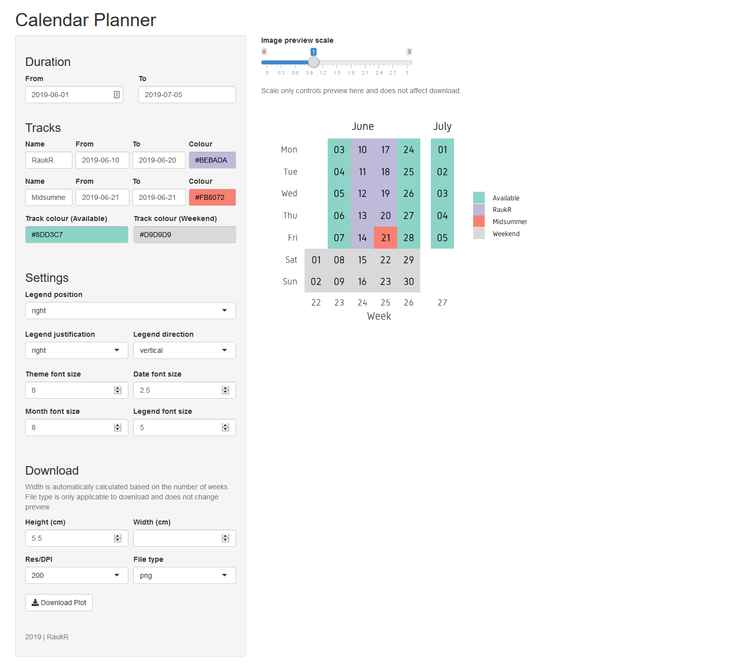
Below is a preview of the finished app.

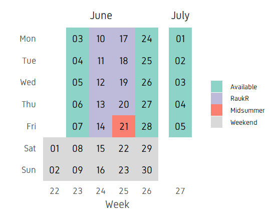
The idea of this app is to create and display a calendar styled planner. Below is a preview of the expected output.

The image is a plot created in ggplot. X axis showing week numbers, y axis showing weekdays, facet titles showing months and dates are colored by categories. We can split this into two parts. The first part is preparing the code for the core task at hand (ie; generating the plot) and the second part is creating a graphical user interface around it using shiny apps to enable the user to input values and adjust dates, categories, plot parameters etc.

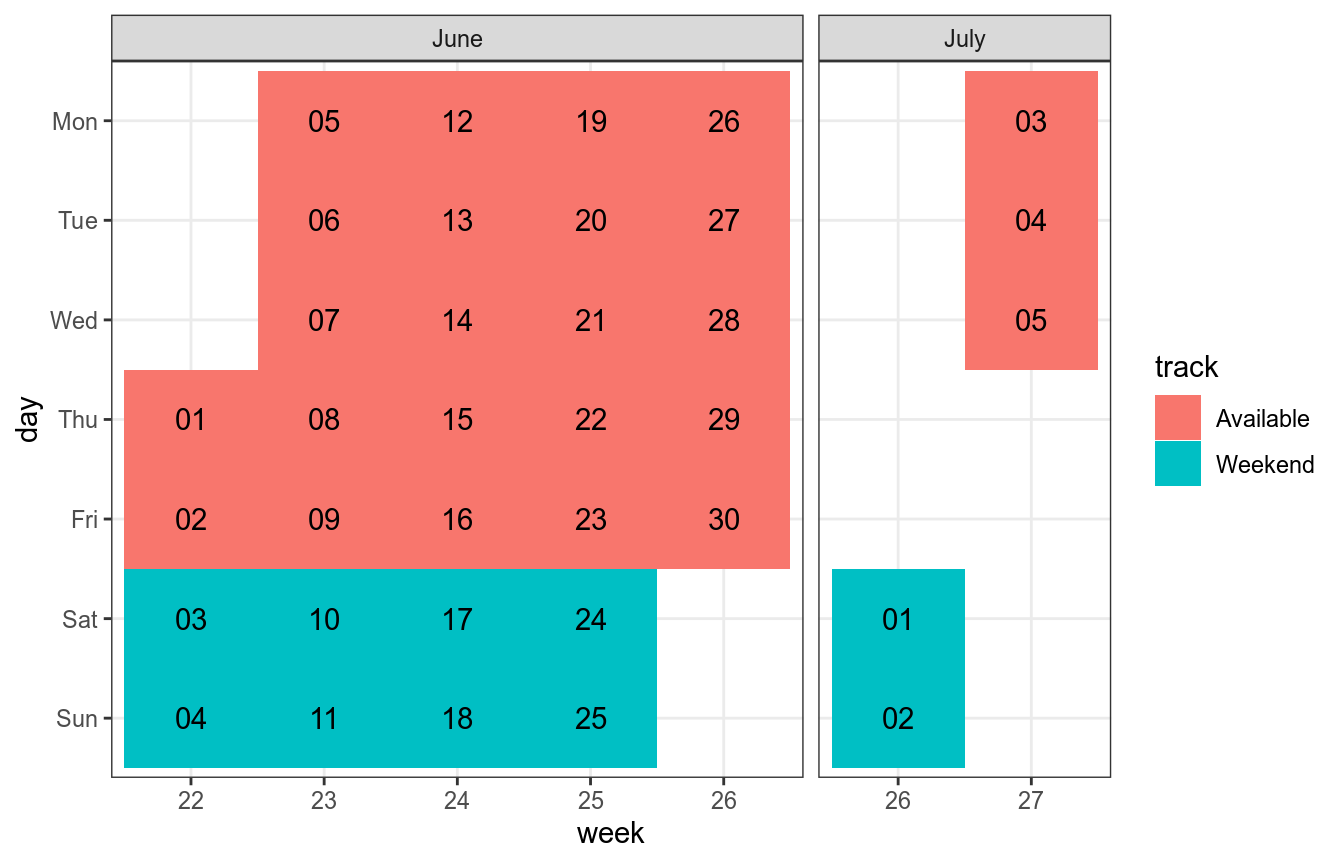
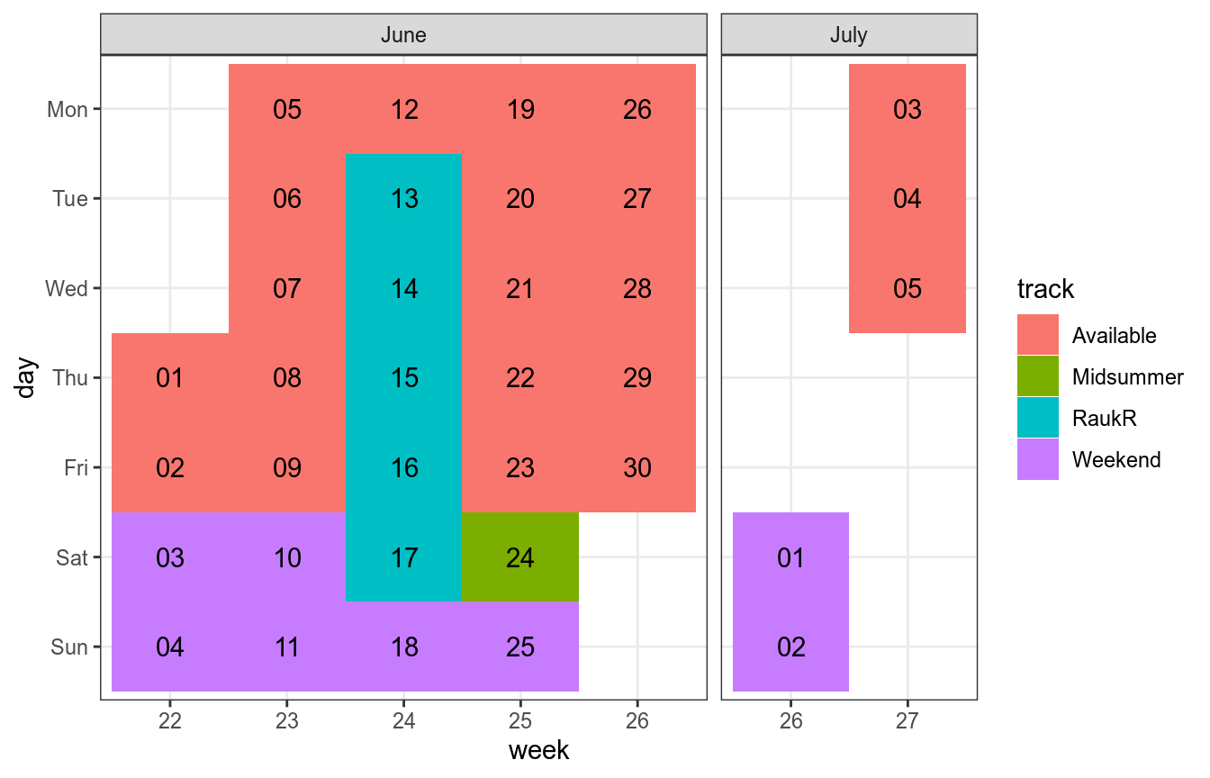
15.1 Creating the plot

The first step is to figure out how to create this plot in ggplot. The data will be contained in a data.frame. The data.frame is created based on start and end dates.

start_date <- as.Date("2023-06-01")
end_date <- as.Date("2023-07-05")
dfr <- data.frame(date=seq(start_date,end_date,by=1))
head(dfr)

date
2023-06-01
2023-06-02
2023-06-03
2023-06-04
2023-06-05
2023-06-06

We can add some code to get specific information from these dates such as the day, week, month and numeric date. Finally we

dfr$day <- factor(strftime(dfr$date,format="%a"),levels=rev(c("Mon","Tue","Wed","Thu","Fri","Sat","Sun")))
dfr$week <- factor(strftime(dfr$date,format="%V"))
dfr$month <- strftime(dfr$date,format="%B")
dfr$month <- factor(dfr$month,levels=unique(dfr$month))
dfr$ddate <- factor(strftime(dfr$date,format="%d"))
head(dfr)

date	day	week	month	ddate
2023-06-01	Thu	22	June	01
2023-06-02	Fri	22	June	02
2023-06-03	Sat	22	June	03
2023-06-04	Sun	22	June	04
2023-06-05	Mon	23	June	05
2023-06-06	Tue	23	June	06

Finally, we add a column called track which will hold the categorical information for colouring dates by activity.

dfr$track <- "Available"
dfr$track[dfr$day=="Sat"|dfr$day=="Sun"] <- "Weekend"
head(dfr)

date	day	week	month	ddate	track
2023-06-01	Thu	22	June	01	Available
2023-06-02	Fri	22	June	02	Available
2023-06-03	Sat	22	June	03	Weekend
2023-06-04	Sun	22	June	04	Weekend
2023-06-05	Mon	23	June	05	Available
2023-06-06	Tue	23	June	06	Available

This is enough information to plot.

ggplot(dfr,aes(x=week,y=day))+
      geom_tile(aes(fill=track))+
      geom_text(aes(label=ddate))+
      facet_grid(~month,scales="free",space="free")+
      theme_bw()

We can add more activities to the track column. Or in other words, I refer to it as adding more tracks.

dfr$track[dfr$date>=as.Date("2023-06-13") & dfr$date<=as.Date("2023-06-17")] <- "RaukR"
dfr$track[dfr$date==as.Date("2023-06-24")] <- "Midsummer"

ggplot(dfr,aes(x=week,y=day))+
      geom_tile(aes(fill=track))+
      geom_text(aes(label=ddate))+
      facet_grid(~month,scales="free",space="free")+
      theme_bw()

Now, we can customize the plot as you prefer. I am modifying the axes labels, changing colors and removing most of the plot elements.

all_cols <- c("#bebada","#fb8072","#80b1d3","#fdb462")
  
ggplot(dfr,aes(x=week,y=day))+
      geom_tile(aes(fill=track))+
      geom_text(aes(label=ddate))+
      scale_fill_manual(values=all_cols)+
      facet_grid(~month,scales="free",space="free")+
      labs(x="Week",y="")+
      theme_bw(base_size=14)+
      theme(legend.title=element_blank(),
            panel.grid=element_blank(),
            panel.border=element_blank(),
            axis.ticks=element_blank(),
            axis.title=element_text(colour="grey30"),
            strip.background=element_blank(),
            legend.key.size=unit(0.3,"cm"),
            legend.spacing.x=unit(0.2,"cm"))

Our plot is now ready and we have the code to create this plot. The next step is to build a shiny app around it.

15.2 Building the app

15.2.1 Layout

We need to first have a plan for the app page, which UI elements to include and how they will be laid out and structured. My plan is as shown in the preview image.

There is a horizontal top bar for the title and two columns below. The left column will contain the input widgets and control. The right column will contain the plot output. Since, this is a commonly used layout, it is available as a predefined function in shiny called pageWithSidebar(). It takes three arguments headerPanel, sidebarPanel and mainPanel which is self explanatory.

shinyApp(
ui=fluidPage(
  pageWithSidebar(
    headerPanel(),
    sidebarPanel(),
    mainPanel())
  ),
server=function(input,output){}
)

15.2.2 UI

Then we fill in the panels with widgets and contents.

shinyApp(
ui=fluidPage(
  pageWithSidebar(
    headerPanel(title="Calendar Planner",windowTitle="Calendar Planner"),
    sidebarPanel(
      h3("Duration"),
      fluidRow(
          column(6,
              dateInput("in_duration_date_start","From",value=format(Sys.time(),"%Y-%m-%d"))
          ),
          column(6,
              dateInput("in_duration_date_end","To",value=format(as.Date(Sys.time())+30,"%Y-%m-%d"))
          )
      )
    ),
    mainPanel())
  ),
server=function(input,output){},
  options=list(height="400px")
)

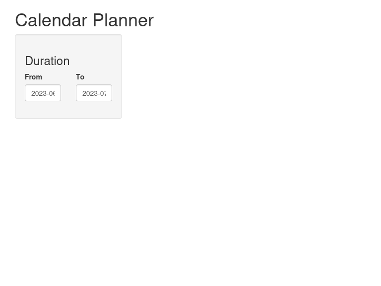
We have defined a part of the side bar panel with a title Duration. fluidRow() is an html tag used to create rows. Above, in the side bar panel, a row is defined and two columns are defined inside. Each column is filled with date input widgets for start and end dates. We use the columns here to place date input widgets side by side. To place widgets one below the other, the columns can simply be removed. The default value for the start date is set to current date and the end date is set to current date + 30 days.

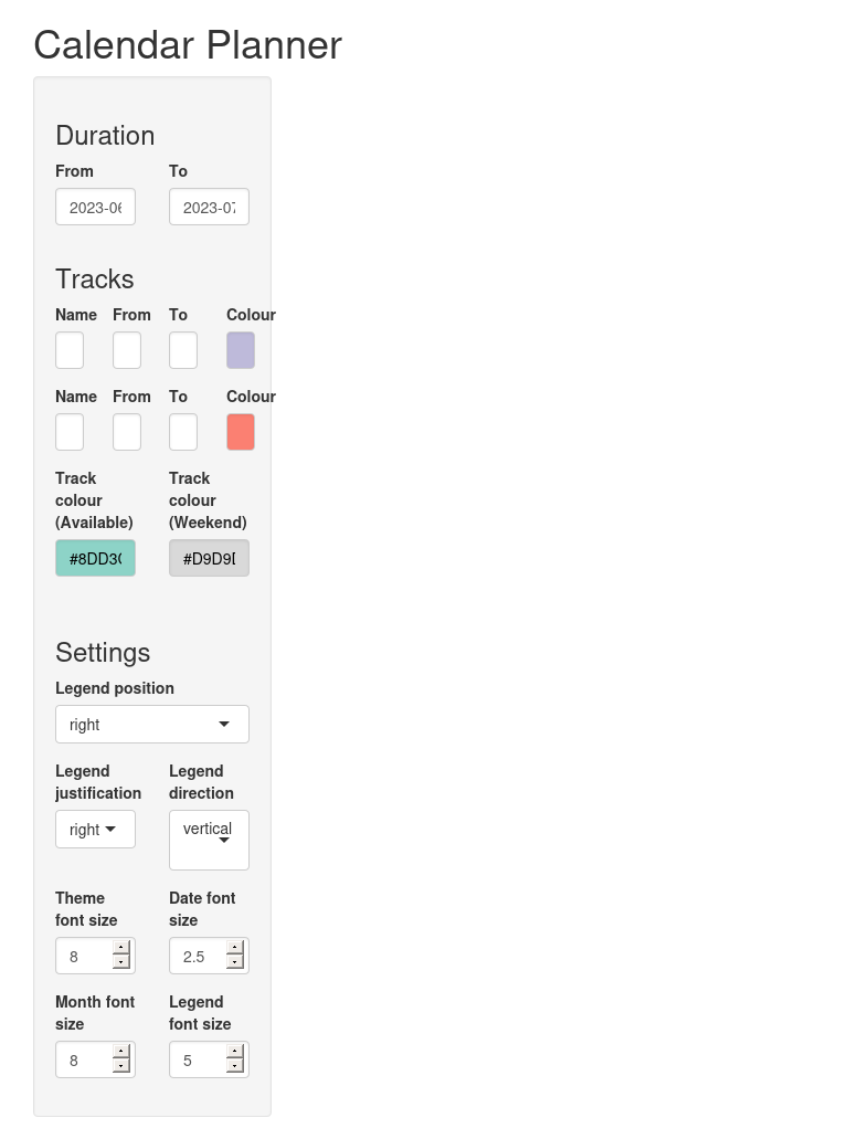
Now we add more sections to the side bar panel, namely track input variables and plot settings variables. We also added custom colors. Custom colors can be selected using the input widget colourpicker::colourInput().

cols <- toupper(c(
  "#bebada","#fb8072","#80b1d3","#fdb462","#b3de69","#fccde5","#FDBF6F","#A6CEE3",
  "#56B4E9","#B2DF8A","#FB9A99","#CAB2D6","#A9C4E2","#79C360","#FDB762","#9471B4",
  "#A4A4A4","#fbb4ae","#b3cde3","#ccebc5","#decbe4","#fed9a6","#ffffcc","#e5d8bd",
  "#fddaec","#f2f2f2","#8dd3c7","#d9d9d9"))
  
shinyApp(
ui=fluidPage(
  pageWithSidebar(
    headerPanel(title="Calendar Planner",windowTitle="Calendar Planner"),
    sidebarPanel(
      h3("Duration"),
      fluidRow(
          column(6,
              dateInput("in_duration_date_start","From",value=format(Sys.time(),"%Y-%m-%d"))
          ),
          column(6,
              dateInput("in_duration_date_end","To",value=format(as.Date(Sys.time())+30,"%Y-%m-%d"))
          )
      ),
      h3("Tracks"),
      fluidRow(
          column(3,
              textInput("in_track_name_1",label="Name",value="Vacation",placeholder="Vacation")
          ),
          column(3,
              dateInput("in_track_date_start_1",label="From",value=format(Sys.time(),"%Y-%m-%d"))
          ),
          column(3,
              dateInput("in_track_date_end_1",label="To",value=format(as.Date(Sys.time())+30,"%Y-%m-%d"))
          ),
          column(3,
              colourpicker::colourInput("in_track_colour_1",label="Colour",
                                        palette="limited",allowedCols=cols,value=cols[1])
          )
      ),
      fluidRow(
          column(3,
              textInput("in_track_name_2",label="Name",value="Offline",placeholder="Offline")
          ),
          column(3,
              dateInput("in_track_date_start_2",label="From",value=format(Sys.time(),"%Y-%m-%d"))
          ),
          column(3,
              dateInput("in_track_date_end_2",label="To",value=format(as.Date(Sys.time())+30,"%Y-%m-%d"))
          ),
          column(3,
              colourpicker::colourInput("in_track_colour_2",label="Colour",
                                        palette="limited",allowedCols=cols,value=cols[2])
          )
      ),
      fluidRow(
          column(6,
              colourpicker::colourInput("in_track_colour_available",label="Track colour (Available)",
                                        palette="limited",allowedCols=cols,value=cols[length(cols)-1])
          ),
          column(6,
              colourpicker::colourInput("in_track_colour_weekend",label="Track colour (Weekend)",
                                        palette="limited",allowedCols=cols,value=cols[length(cols)])
          )
      ),
      tags$br(),
      h3("Settings"),
      selectInput("in_legend_position",label="Legend position",
                  choices=c("top","right","left","bottom"),selected="right",multiple=F),
      fluidRow(
          column(6,
              selectInput("in_legend_justification",label="Legend justification",
                          choices=c("left","right"),selected="right",multiple=F)
          ),
          column(6,
              selectInput("in_legend_direction",label="Legend direction",
                          choices=c("vertical","horizontal"),selected="vertical",multiple=F)
          )
      ),
      fluidRow(
          column(6,
              numericInput("in_themefontsize",label="Theme font size",value=8,step=0.5)
          ),
          column(6,
              numericInput("in_datefontsize",label="Date font size",value=2.5,step=0.1)
          )
      ),
      fluidRow(
          column(6,
              numericInput("in_monthfontsize",label="Month font size",value=8,step=0.5)
          ),
          column(6,
              numericInput("in_legendfontsize",label="Legend font size",value=5,step=0.5)
          )
      )
    ),
    mainPanel(
      plotOutput("out_plot")
    ))
  ),
server=function(input,output){}
)

The track start and end dates are by default set to the same as that of duration start and end dates. We will adjust this later. Under the settings section, we have added a few useful plot variables to adjust sizes and spacing of plot elements. They are set to reasonable defaults. These variables will be passed on to the ggplot plotting function.

We can end with column with the download options. Input fields are height, width, resolution and file format. Last we add a button for download.

h3("Download"),
helpText("Width is automatically calculated based on the number of weeks. File type is only applicable to download and does not change preview."),
fluidRow(
    column(6,
        numericInput("in_height","Height (cm)",step=0.5,value=5.5)
    ),
    column(6,
        numericInput("in_width","Width (cm)",step=0.5,value=NA)
    )
),
fluidRow(
    column(6,
        selectInput("in_res","Res/DPI",choices=c("200","300","400","500"),selected="200")
    ),
    column(6,
        selectInput("in_format","File type",choices=c("png","tiff","jpeg","pdf"),selected="png",multiple=FALSE,selectize=TRUE)
    )
),
downloadButton("btn_downloadplot","Download Plot"),
tags$hr(),
helpText("RaukR")

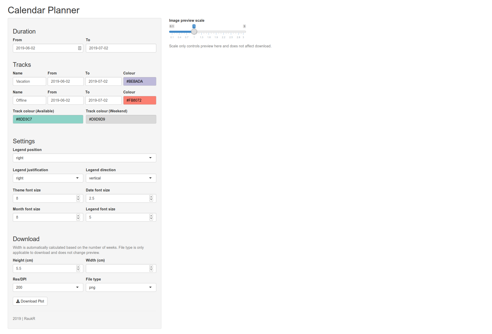
In the main panel, we add the plot output function that will hold the output plot. We also add a slider for image preview scaling and the output image. The idea behind the preview scaling is to allow the user to increase or decrease the size of the plot in the browser without affecting the download size. The part of the UI code to add the preview slider is below:

mainPanel(
  sliderInput("in_scale","Image preview scale",min=0.1,max=3,step=0.10,value=1),
  helpText("Scale only controls preview here and does not affect download."),
  tags$br(),
  imageOutput("out_plot")
)

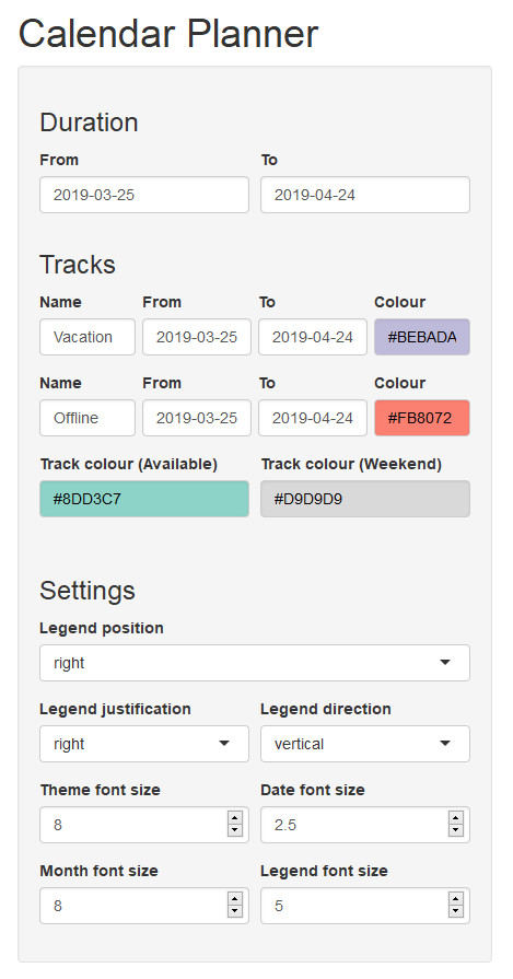
This should now look like this. Some additional styling has been added to divs.

## load colours
cols <- toupper(c(
  "#bebada","#fb8072","#80b1d3","#fdb462","#b3de69","#fccde5","#FDBF6F","#A6CEE3",
  "#56B4E9","#B2DF8A","#FB9A99","#CAB2D6","#A9C4E2","#79C360","#FDB762","#9471B4",
  "#A4A4A4","#fbb4ae","#b3cde3","#ccebc5","#decbe4","#fed9a6","#ffffcc","#e5d8bd",
  "#fddaec","#f2f2f2","#8dd3c7","#d9d9d9"))

shinyApp(
  ui=fluidPage(
    pageWithSidebar(
      headerPanel(title="Calendar Planner",windowTitle="Calendar Planner"),
      sidebarPanel(
        h3("Duration"),
        fluidRow(
          column(6,style=list("padding-right: 5px;"),
                 dateInput("in_duration_date_start","From",value=format(Sys.time(),"%Y-%m-%d"))
          ),
          column(6,style=list("padding-left: 5px;"),
                 dateInput("in_duration_date_end","To",value=format(as.Date(Sys.time())+30,"%Y-%m-%d"))
          )
        ),
        h3("Tracks"),
        fluidRow(
          column(3,style=list("padding-right: 3px;"),
                 textInput("in_track_name_1",label="Name",value="Vacation",placeholder="Vacation")
          ),
          column(3,style=list("padding-right: 3px; padding-left: 3px;"),
                 dateInput("in_track_date_start_1",label="From",value=format(Sys.time(),"%Y-%m-%d"))
          ),
          column(3,style=list("padding-right: 3px; padding-left: 3px;"),
                 dateInput("in_track_date_end_1",label="To",value=format(as.Date(Sys.time())+30,"%Y-%m-%d"))
          ),
          column(3,style=list("padding-left: 3px;"),
                 colourpicker::colourInput("in_track_colour_1",label="Colour",
                                           palette="limited",allowedCols=cols,value=cols[1])
          )
        ),
        fluidRow(
          column(3,style=list("padding-right: 3px;"),
                 textInput("in_track_name_2",label="Name",value="Offline",placeholder="Offline")
          ),
          column(3,style=list("padding-right: 3px; padding-left: 3px;"),
                 dateInput("in_track_date_start_2",label="From",value=format(Sys.time(),"%Y-%m-%d"))
          ),
          column(3,style=list("padding-right: 3px; padding-left: 3px;"),
                 dateInput("in_track_date_end_2",label="To",value=format(as.Date(Sys.time())+30,"%Y-%m-%d"))
          ),
          column(3,style=list("padding-left: 3px;"),
                 colourpicker::colourInput("in_track_colour_2",label="Colour",
                                           palette="limited",allowedCols=cols,value=cols[2])
          )
        ),
        fluidRow(
          column(6,style=list("padding-right: 5px;"),
                 colourpicker::colourInput("in_track_colour_available",label="Track colour (Available)",
                                           palette="limited",allowedCols=cols,value=cols[length(cols)-1])
          ),
          column(6,style=list("padding-left: 5px;"),
                 colourpicker::colourInput("in_track_colour_weekend",label="Track colour (Weekend)",
                                           palette="limited",allowedCols=cols,value=cols[length(cols)])
          )
        ),
        tags$br(),
        h3("Settings"),
        selectInput("in_legend_position",label="Legend position",
                    choices=c("top","right","left","bottom"),selected="right",multiple=F),
        fluidRow(
          column(6,style=list("padding-right: 5px;"),
                 selectInput("in_legend_justification",label="Legend justification",
                             choices=c("left","right"),selected="right",multiple=F)
          ),
          column(6,style=list("padding-left: 5px;"),
                 selectInput("in_legend_direction",label="Legend direction",
                             choices=c("vertical","horizontal"),selected="vertical",multiple=F)
          )
        ),
        fluidRow(
          column(6,style=list("padding-right: 5px;"),
                 numericInput("in_themefontsize",label="Theme font size",value=8,step=0.5)
          ),
          column(6,style=list("padding-left: 5px;"),
                 numericInput("in_datefontsize",label="Date font size",value=2.5,step=0.1)
          )
        ),
        fluidRow(
          column(6,style=list("padding-right: 5px;"),
                 numericInput("in_monthfontsize",label="Month font size",value=8,step=0.5)
          ),
          column(6,style=list("padding-left: 5px;"),
                 numericInput("in_legendfontsize",label="Legend font size",value=5,step=0.5)
          )
        ),
        tags$br(),
        h3("Download"),
        helpText("Width is automatically calculated based on the number of weeks. File type is only applicable to download and does not change preview."),
        fluidRow(
          column(6,style=list("padding-right: 5px;"),
                 numericInput("in_height","Height (cm)",step=0.5,value=5.5)
          ),
          column(6,style=list("padding-left: 5px;"),
                 numericInput("in_width","Width (cm)",step=0.5,value=NA)
          )
        ),
        fluidRow(
          column(6,style=list("padding-right: 5px;"),
                 selectInput("in_res","Res/DPI",choices=c("200","300","400","500"),selected="200")
          ),
          column(6,style=list("padding-left: 5px;"),
                 selectInput("in_format","File type",choices=c("png","tiff","jpeg","pdf"),selected="png",multiple=FALSE,selectize=TRUE)
          )
        ),
        downloadButton("btn_downloadplot","Download Plot"),
        tags$hr(),
        helpText("RaukR")
      ),
      mainPanel(
        sliderInput("in_scale","Image preview scale",min=0.1,max=3,step=0.10,value=1),
        helpText("Scale only controls preview here and does not affect download."),
        tags$br(),
        imageOutput("out_plot")
      )
    )
  ),
  server=function(input,output){}
)

15.2.3 Server

We can start adding content into the server function to actually enable functionality.

The server code can be organized into 5 blocks.

1. fn_plot(): Reactive function that generates ggplot object
2. out_plot: Plots the ggplot object
3. fn_downloadplotname(): Function to create download image name
4. fn_downloadplot(): Function to create and download the image
5. btn_downloadplot: Download handler that runs fn_downloadplot on button trigger
6. observe: Observer that updates input values

Here is a flow diagram of how these blocks work.

     1 > [2]
     v
3 > [4] < 5

    {6}

The core block 1 creates the preview plot in block 2. The download handler block 5 calls block 1 to generate the plot which is downloaded using block 4. Block 6 is standalone observer.

Reactive values used across multiple functions can be stored using reactiveValues(). These can be written to or accessed from within a reactive environment.

store <- reactiveValues(week=NULL)

We have our core function fn_plot() (block 1). Inputs are validated and gathered from input widgets. We are using shiny::req() to silently check that necessary input variables are available before running through the function. We use validate() with need() to run some basic sanity checks namely that track names are not duplicated and to ensure that start-dates precede end-dates. Necessary date-time calculations are performed. The calendar plot is created and returned.

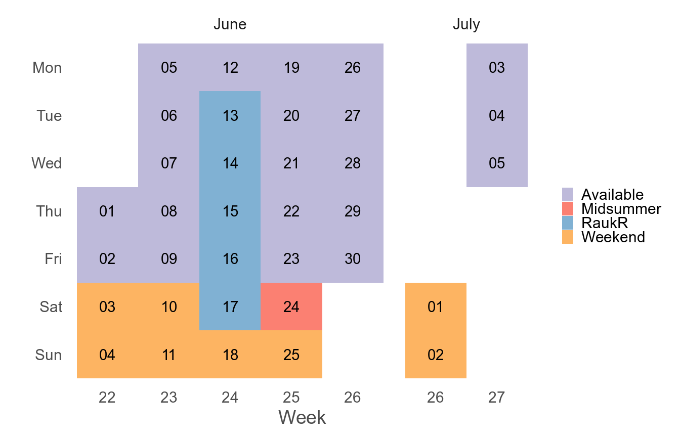
## RFN: fn_plot -----------------------------------------------------------
## core plotting function, returns a ggplot object

fn_plot <- reactive({

  shiny::req(input$in_duration_date_start)
  shiny::req(input$in_duration_date_end)

  shiny::req(input$in_track_date_start_1)
  shiny::req(input$in_track_date_end_1)
  shiny::req(input$in_track_name_1)
  shiny::req(input$in_track_colour_1)

  shiny::req(input$in_track_date_start_2)
  shiny::req(input$in_track_date_end_2)
  shiny::req(input$in_track_name_2)
  shiny::req(input$in_track_colour_2)

  shiny::req(input$in_legend_position)
  shiny::req(input$in_legend_justification)
  shiny::req(input$in_legend_direction)
  shiny::req(input$in_themefontsize)
  shiny::req(input$in_datefontsize)
  shiny::req(input$in_monthfontsize)
  shiny::req(input$in_legendfontsize)

  validate(need(input$in_track_name_1!=input$in_track_name_2,"Duplicate track names are not allowed."))
  validate(need(as.Date(input$in_duration_date_start) < as.Date(input$in_duration_date_end),"End duration date must be later than start duration date."))

  # prepare dates
  dfr <- data.frame(date=seq(as.Date(input$in_duration_date_start),as.Date(input$in_duration_date_end),by=1))
  dfr$day <- factor(strftime(dfr$date,format="%a"),levels=rev(c("Mon","Tue","Wed","Thu","Fri","Sat","Sun")))
  dfr$week <- factor(strftime(dfr$date,format="%V"))
  dfr$month <- strftime(dfr$date,format="%B")
  dfr$month <- factor(dfr$month,levels=unique(dfr$month))
  dfr$ddate <- factor(strftime(dfr$date,format="%d"))

  #add tracks
  dfr$track <- "Available"
  dfr$track[dfr$day=="Sat" | dfr$day=="Sun"] <- "Weekend"

  temp_start_date_1 <- as.Date(input$in_track_date_start_1)
  temp_end_date_1 <- as.Date(input$in_track_date_end_1)
  temp_track_name_1 <- input$in_track_name_1
  temp_track_col_1 <- input$in_track_colour_1
  validate(need(temp_start_date_1 < temp_end_date_1,"End track duration date must be later than start track duration date."))
  dfr$track[dfr$date>=temp_start_date_1 & dfr$date<=temp_end_date_1] <- temp_track_name_1

  temp_start_date_2 <- as.Date(input$in_track_date_start_2)
  temp_end_date_2 <- as.Date(input$in_track_date_end_2)
  temp_track_name_2 <- input$in_track_name_2
  temp_track_col_2 <- input$in_track_colour_2
  validate(need(temp_start_date_2 < temp_end_date_2,"End track duration date must be later than start track duration date."))
  dfr$track[dfr$date>=temp_start_date_2 & dfr$date<=temp_end_date_2] <- temp_track_name_2

  # create order factor
  fc <- vector(mode="character")
  if("Available" %in% unique(dfr$track)) fc <- c(fc,"Available")
  fc <- c(fc,temp_track_name_1,temp_track_name_2)
  if("Weekend" %in% unique(dfr$track)) fc <- c(fc,"Weekend")
  dfr$track <- factor(dfr$track,levels=fc)

  # prepare colours
  all_cols <- c(input$in_track_colour_available,temp_track_col_1,temp_track_col_2,input$in_track_colour_weekend)

  # plot
  p <- ggplot(dfr,aes(x=week,y=day))+
    geom_tile(aes(fill=track))+
    geom_text(aes(label=ddate),size=input$in_datefontsize)+
    scale_fill_manual(values=all_cols)+
    facet_grid(~month,scales="free",space="free")+
    labs(x="Week",y="")+
    theme_bw(base_size=input$in_themefontsize)+
    theme(legend.title=element_blank(),
          panel.grid=element_blank(),
          panel.border=element_blank(),
          axis.ticks=element_blank(),
          axis.title=element_text(colour="grey30"),
          strip.background=element_blank(),
          strip.text=element_text(size=input$in_monthfontsize),
          legend.position=input$in_legend_position,
          legend.justification=input$in_legend_justification,
          legend.direction=input$in_legend_direction,
          legend.text=element_text(size=input$in_legendfontsize),
          legend.key.size=unit(0.3,"cm"),
          legend.spacing.x=unit(0.2,"cm"))

  # add number of weeks to reactive value
  store$week <- length(levels(dfr$week))

  return(p)
})

Here is the block that generates the output image. Image dimensions and resolution is obtained from input widgets. Default width is computed based on number of weeks. This is why the number of weeks was stored as a reactive value. The plot is exported to the working directly and then displayed in the browser. The scale slider allows the plot preview to be scaled in the browser.

## OUT: out_plot ------------------------------------------------------------
## plots figure

output$out_plot <- renderImage({

  shiny::req(fn_plot())
  shiny::req(input$in_height)
  shiny::req(input$in_res)
  shiny::req(input$in_scale)

  height <- as.numeric(input$in_height)
  width <- as.numeric(input$in_width)
  res <- as.numeric(input$in_res)

  if(is.na(width)) {
    width <- (store$week*1.2)
    if(width < 4.5) width <- 4.5
  }

  p <- fn_plot()
  ggsave("calendar_plot.png",p,height=height,width=width,units="cm",dpi=res)

  return(list(src="calendar_plot.png",
              contentType="image/png",
              width=round(((width*res)/2.54)*input$in_scale,0),
              height=round(((height*res)/2.54)*input$in_scale,0),
              alt="calendar_plot"))
}, deleteFile=TRUE)

The fn_downloadplotname() function simply generates the output filename depending on the filetype extension.

# FN: fn_downloadplotname ----------------------------------------------------
# creates filename for download plot

fn_downloadplotname <- function()
{
  return(paste0("calendar_plot.",input$in_format))
}

The fn_downloadplot() function uses fn_plot() to create the image and then export the image.

## FN: fn_downloadplot -------------------------------------------------
## function to download plot

fn_downloadplot <- function(){
  shiny::req(fn_plot())
  shiny::req(input$in_height)
  shiny::req(input$in_res)
  shiny::req(input$in_scale)

  height <- as.numeric(input$in_height)
  width <- as.numeric(input$in_width)
  res <- as.numeric(input$in_res)
  format <- input$in_format

  if(is.na(width)) width <- (store$week*1)+1

  p <- fn_plot()
  if(format=="pdf" | format=="svg"){
    ggsave(fn_downloadplotname(),p,height=height,width=width,units="cm",dpi=res)
    #embed_fonts(fn_downloadplotname())
  }else{
    ggsave(fn_downloadplotname(),p,height=height,width=width,units="cm",dpi=res)
  }
}

The download handler then downloads the file.

## DHL: btn_downloadplot ----------------------------------------------------
## download handler for downloading plot

output$btn_downloadplot <- downloadHandler(
  filename=fn_downloadplotname,
  content=function(file) {
    fn_downloadplot()
    file.copy(fn_downloadplotname(),file,overwrite=T)
  }
)

Finally, we have the observer function. The observer continuously monitors change in input widgets of interest (here start and end duration) and updates other widget values.

## OBS: tracks dates ---------------------------------------------------------

observe({
  
  shiny::req(input$in_duration_date_start)
  shiny::req(input$in_duration_date_end)
  
  validate(need(as.Date(input$in_duration_date_start) < as.Date(input$in_duration_date_end),"End duration date must be later than start duration date."))
  
  # create date intervals
  dseq <- seq(as.Date(input$in_duration_date_start),as.Date(input$in_duration_date_end),by=1)
  r1 <- unique(as.character(cut(dseq,breaks=3)))
  
  updateDateInput(session,"in_track_date_start_1",label="From",value=as.Date(r1[1],"%Y-%m-%d"))
  updateDateInput(session,"in_track_date_end_1",label="To",value=as.Date(r1[1+1],"%Y-%m-%d")-1)
  updateDateInput(session,"in_track_date_start_2",label="From",value=as.Date(r1[2],"%Y-%m-%d"))
  updateDateInput(session,"in_track_date_end_2",label="To",value=as.Date(r1[2+1],"%Y-%m-%d")-1)
  
})

The complete code for the app is as below.

## load libraries
library(ggplot2)
library(shiny)
library(colourpicker)

## load colours
cols <- toupper(c(
  "#bebada","#fb8072","#80b1d3","#fdb462","#b3de69","#fccde5","#FDBF6F","#A6CEE3",
  "#56B4E9","#B2DF8A","#FB9A99","#CAB2D6","#A9C4E2","#79C360","#FDB762","#9471B4",
  "#A4A4A4","#fbb4ae","#b3cde3","#ccebc5","#decbe4","#fed9a6","#ffffcc","#e5d8bd",
  "#fddaec","#f2f2f2","#8dd3c7","#d9d9d9"))

shinyApp(

# UI ---------------------------------------------------------------------------

ui=fluidPage(
  pageWithSidebar(
    headerPanel(title="Calendar Planner",windowTitle="Calendar Planner"),
    sidebarPanel(
      h3("Duration"),
      fluidRow(
          column(6,style=list("padding-right: 5px;"),
              dateInput("in_duration_date_start","From",value=format(Sys.time(),"%Y-%m-%d"))
          ),
          column(6,style=list("padding-left: 5px;"),
              dateInput("in_duration_date_end","To",value=format(as.Date(Sys.time())+30,"%Y-%m-%d"))
          )
      ),
      h3("Tracks"),
      fluidRow(
          column(3,style=list("padding-right: 3px;"),
              textInput("in_track_name_1",label="Name",value="Vacation",placeholder="Vacation")
          ),
          column(3,style=list("padding-right: 3px; padding-left: 3px;"),
              dateInput("in_track_date_start_1",label="From",value=format(Sys.time(),"%Y-%m-%d"))
          ),
          column(3,style=list("padding-right: 3px; padding-left: 3px;"),
              dateInput("in_track_date_end_1",label="To",value=format(as.Date(Sys.time())+30,"%Y-%m-%d"))
          ),
          column(3,style=list("padding-left: 3px;"),
              colourpicker::colourInput("in_track_colour_1",label="Colour",
                                        palette="limited",allowedCols=cols,value=cols[1])
          )
      ),
      fluidRow(
          column(3,style=list("padding-right: 3px;"),
              textInput("in_track_name_2",label="Name",value="Offline",placeholder="Offline")
          ),
          column(3,style=list("padding-right: 3px; padding-left: 3px;"),
              dateInput("in_track_date_start_2",label="From",value=format(Sys.time(),"%Y-%m-%d"))
          ),
          column(3,style=list("padding-right: 3px; padding-left: 3px;"),
              dateInput("in_track_date_end_2",label="To",value=format(as.Date(Sys.time())+30,"%Y-%m-%d"))
          ),
          column(3,style=list("padding-left: 3px;"),
              colourpicker::colourInput("in_track_colour_2",label="Colour",
                                        palette="limited",allowedCols=cols,value=cols[2])
          )
      ),
      fluidRow(
          column(6,style=list("padding-right: 5px;"),
              colourpicker::colourInput("in_track_colour_available",label="Track colour (Available)",
                                        palette="limited",allowedCols=cols,value=cols[length(cols)-1])
          ),
          column(6,style=list("padding-left: 5px;"),
              colourpicker::colourInput("in_track_colour_weekend",label="Track colour (Weekend)",
                                        palette="limited",allowedCols=cols,value=cols[length(cols)])
          )
      ),
      tags$br(),
      h3("Settings"),
      selectInput("in_legend_position",label="Legend position",
                  choices=c("top","right","left","bottom"),selected="right",multiple=F),
      fluidRow(
          column(6,style=list("padding-right: 5px;"),
              selectInput("in_legend_justification",label="Legend justification",
                          choices=c("left","right"),selected="right",multiple=F)
          ),
          column(6,style=list("padding-left: 5px;"),
              selectInput("in_legend_direction",label="Legend direction",
                          choices=c("vertical","horizontal"),selected="vertical",multiple=F)
          )
      ),
      fluidRow(
          column(6,style=list("padding-right: 5px;"),
              numericInput("in_themefontsize",label="Theme font size",value=8,step=0.5)
          ),
          column(6,style=list("padding-left: 5px;"),
              numericInput("in_datefontsize",label="Date font size",value=2.5,step=0.1)
          )
      ),
      fluidRow(
          column(6,style=list("padding-right: 5px;"),
              numericInput("in_monthfontsize",label="Month font size",value=8,step=0.5)
          ),
          column(6,style=list("padding-left: 5px;"),
              numericInput("in_legendfontsize",label="Legend font size",value=5,step=0.5)
          )
      ),
      tags$br(),
      h3("Download"),
      helpText("Width is automatically calculated based on the number of weeks. File type is only applicable to download and does not change preview."),
      fluidRow(
          column(6,style=list("padding-right: 5px;"),
              numericInput("in_height","Height (cm)",step=0.5,value=5.5)
          ),
          column(6,style=list("padding-left: 5px;"),
              numericInput("in_width","Width (cm)",step=0.5,value=NA)
          )
      ),
      fluidRow(
          column(6,style=list("padding-right: 5px;"),
              selectInput("in_res","Res/DPI",choices=c("200","300","400","500"),selected="200")
          ),
          column(6,style=list("padding-left: 5px;"),
              selectInput("in_format","File type",choices=c("png","tiff","jpeg","pdf"),selected="png",multiple=FALSE,selectize=TRUE)
          )
      ),
      downloadButton("btn_downloadplot","Download Plot"),
      tags$hr(),
      helpText("RaukR")
    ),
    mainPanel(
      sliderInput("in_scale","Image preview scale",min=0.1,max=3,step=0.10,value=1),
      helpText("Scale only controls preview here and does not affect download."),
      tags$br(),
      imageOutput("out_plot")
    )
  )
),

# SERVER -----------------------------------------------------------------------

server=function(input, output, session) {

  store <- reactiveValues(week=NULL)

  ## RFN: fn_plot -----------------------------------------------------------
  ## core plotting function, returns a ggplot object

  fn_plot <- reactive({

    shiny::req(input$in_duration_date_start)
    shiny::req(input$in_duration_date_end)

    shiny::req(input$in_track_date_start_1)
    shiny::req(input$in_track_date_end_1)
    shiny::req(input$in_track_name_1)
    shiny::req(input$in_track_colour_1)

    shiny::req(input$in_track_date_start_2)
    shiny::req(input$in_track_date_end_2)
    shiny::req(input$in_track_name_2)
    shiny::req(input$in_track_colour_2)

    shiny::req(input$in_legend_position)
    shiny::req(input$in_legend_justification)
    shiny::req(input$in_legend_direction)
    shiny::req(input$in_themefontsize)
    shiny::req(input$in_datefontsize)
    shiny::req(input$in_monthfontsize)
    shiny::req(input$in_legendfontsize)

    validate(need(input$in_track_name_1!=input$in_track_name_2,"Duplicate track names are not allowed."))
    validate(need(as.Date(input$in_duration_date_start) < as.Date(input$in_duration_date_end),"End duration date must be later than start duration date."))

    # prepare dates
    dfr <- data.frame(date=seq(as.Date(input$in_duration_date_start),as.Date(input$in_duration_date_end),by=1))
    dfr$day <- factor(strftime(dfr$date,format="%a"),levels=rev(c("Mon","Tue","Wed","Thu","Fri","Sat","Sun")))
    dfr$week <- factor(strftime(dfr$date,format="%V"))
    dfr$month <- strftime(dfr$date,format="%B")
    dfr$month <- factor(dfr$month,levels=unique(dfr$month))
    dfr$ddate <- factor(strftime(dfr$date,format="%d"))

    #add tracks
    dfr$track <- "Available"
    dfr$track[dfr$day=="Sat" | dfr$day=="Sun"] <- "Weekend"

    temp_start_date_1 <- as.Date(input$in_track_date_start_1)
    temp_end_date_1 <- as.Date(input$in_track_date_end_1)
    temp_track_name_1 <- input$in_track_name_1
    temp_track_col_1 <- input$in_track_colour_1
    validate(need(temp_start_date_1 < temp_end_date_1,"End track duration date must be later than start track duration date."))
    dfr$track[dfr$date>=temp_start_date_1 & dfr$date<=temp_end_date_1] <- temp_track_name_1

    temp_start_date_2 <- as.Date(input$in_track_date_start_2)
    temp_end_date_2 <- as.Date(input$in_track_date_end_2)
    temp_track_name_2 <- input$in_track_name_2
    temp_track_col_2 <- input$in_track_colour_2
    validate(need(temp_start_date_2 < temp_end_date_2,"End track duration date must be later than start track duration date."))
    dfr$track[dfr$date>=temp_start_date_2 & dfr$date<=temp_end_date_2] <- temp_track_name_2

    # create order factor
    fc <- vector(mode="character")
    if("Available" %in% unique(dfr$track)) fc <- c(fc,"Available")
    fc <- c(fc,temp_track_name_1,temp_track_name_2)
    if("Weekend" %in% unique(dfr$track)) fc <- c(fc,"Weekend")
    dfr$track <- factor(dfr$track,levels=fc)

    # prepare colours
    all_cols <- c(input$in_track_colour_available,temp_track_col_1,temp_track_col_2,input$in_track_colour_weekend)

    # plot
    p <- ggplot(dfr,aes(x=week,y=day))+
      geom_tile(aes(fill=track))+
      geom_text(aes(label=ddate),size=input$in_datefontsize)+
      scale_fill_manual(values=all_cols)+
      facet_grid(~month,scales="free",space="free")+
      labs(x="Week",y="")+
      theme_bw(base_size=input$in_themefontsize)+
      theme(legend.title=element_blank(),
            panel.grid=element_blank(),
            panel.border=element_blank(),
            axis.ticks=element_blank(),
            axis.title=element_text(colour="grey30"),
            strip.background=element_blank(),
            strip.text=element_text(size=input$in_monthfontsize),
            legend.position=input$in_legend_position,
            legend.justification=input$in_legend_justification,
            legend.direction=input$in_legend_direction,
            legend.text=element_text(size=input$in_legendfontsize),
            legend.key.size=unit(0.3,"cm"),
            legend.spacing.x=unit(0.2,"cm"))

    # add number of weeks to reactive value
    store$week <- length(levels(dfr$week))

    return(p)
  })

  ## OUT: out_plot ------------------------------------------------------------
  ## plots figure

  output$out_plot <- renderImage({

    shiny::req(fn_plot())
    shiny::req(input$in_height)
    shiny::req(input$in_res)
    shiny::req(input$in_scale)

    height <- as.numeric(input$in_height)
    width <- as.numeric(input$in_width)
    res <- as.numeric(input$in_res)

    if(is.na(width)) {
      width <- (store$week*1.2)
      if(width < 4.5) width <- 4.5
    }

    p <- fn_plot()
    ggsave("calendar_plot.png",p,height=height,width=width,units="cm",dpi=res)

    return(list(src="calendar_plot.png",
                contentType="image/png",
                width=round(((width*res)/2.54)*input$in_scale,0),
                height=round(((height*res)/2.54)*input$in_scale,0),
                alt="calendar_plot"))
  }, deleteFile=TRUE)

  # FN: fn_downloadplotname ----------------------------------------------------
  # creates filename for download plot

  fn_downloadplotname <- function()
  {
    return(paste0("calendar_plot.",input$in_format))
  }

  ## FN: fn_downloadplot -------------------------------------------------
  ## function to download plot

  fn_downloadplot <- function(){
    shiny::req(fn_plot())
    shiny::req(input$in_height)
    shiny::req(input$in_res)
    shiny::req(input$in_scale)

    height <- as.numeric(input$in_height)
    width <- as.numeric(input$in_width)
    res <- as.numeric(input$in_res)
    format <- input$in_format

    if(is.na(width)) width <- (store$week*1)+1

    p <- fn_plot()
    if(format=="pdf" | format=="svg"){
      ggsave(fn_downloadplotname(),p,height=height,width=width,units="cm",dpi=res)
      #embed_fonts(fn_downloadplotname())
    }else{
      ggsave(fn_downloadplotname(),p,height=height,width=width,units="cm",dpi=res)

    }
  }

  ## DHL: btn_downloadplot ----------------------------------------------------
  ## download handler for downloading plot

  output$btn_downloadplot <- downloadHandler(
    filename=fn_downloadplotname,
    content=function(file) {
      fn_downloadplot()
      file.copy(fn_downloadplotname(),file,overwrite=T)
    }
  )

  ## OBS: tracks dates ---------------------------------------------------------
  
  observe({
    
    shiny::req(input$in_duration_date_start)
    shiny::req(input$in_duration_date_end)
    
    validate(need(as.Date(input$in_duration_date_start) < as.Date(input$in_duration_date_end),"End duration date must be later than start duration date."))
    
    # create date intervals
    dseq <- seq(as.Date(input$in_duration_date_start),as.Date(input$in_duration_date_end),by=1)
    r1 <- unique(as.character(cut(dseq,breaks=3)))
    
    updateDateInput(session,"in_track_date_start_1",label="From",value=as.Date(r1[1],"%Y-%m-%d"))
    updateDateInput(session,"in_track_date_end_1",label="To",value=as.Date(r1[1+1],"%Y-%m-%d")-1)
    updateDateInput(session,"in_track_date_start_2",label="From",value=as.Date(r1[2],"%Y-%m-%d"))
    updateDateInput(session,"in_track_date_end_2",label="To",value=as.Date(r1[2+1],"%Y-%m-%d")-1)
    
  })
})

Hopefully, this has not been too overwhelming. Shiny app code may look over-complicated on the first look, but it is easier to understand what is happening by breaking it apart into smaller chunks and understanding how the various components are connected. It is crucial to plan out the structure of your app well in advanced as it is easy to get confused. Remember to name functions and variables sensibly. Use text output widgets and/or print statements in the code to keep track of internal variable values during run-time. Go forth and build awesome apps!