library(reticulate)
library(keras)
# keras::install_keras()
# OR
# keras::install_keras(method="conda", envname="keras")
# OR
# reticulate::conda_install("keras",c("keras","tensorflow"))
Note
In this lab we will learn to code an Artificial Neural Network (ANN) in R both from scratch and using Keras / Tensorflow library. For simplicity, we consider a problem of linearly separable two classes of data points.
Warning
Setting up keras properly might be tricky depending on your OS and setup.
Load the keras library and install keras and tensorflow in the same environment as R.
1 Problem formulation
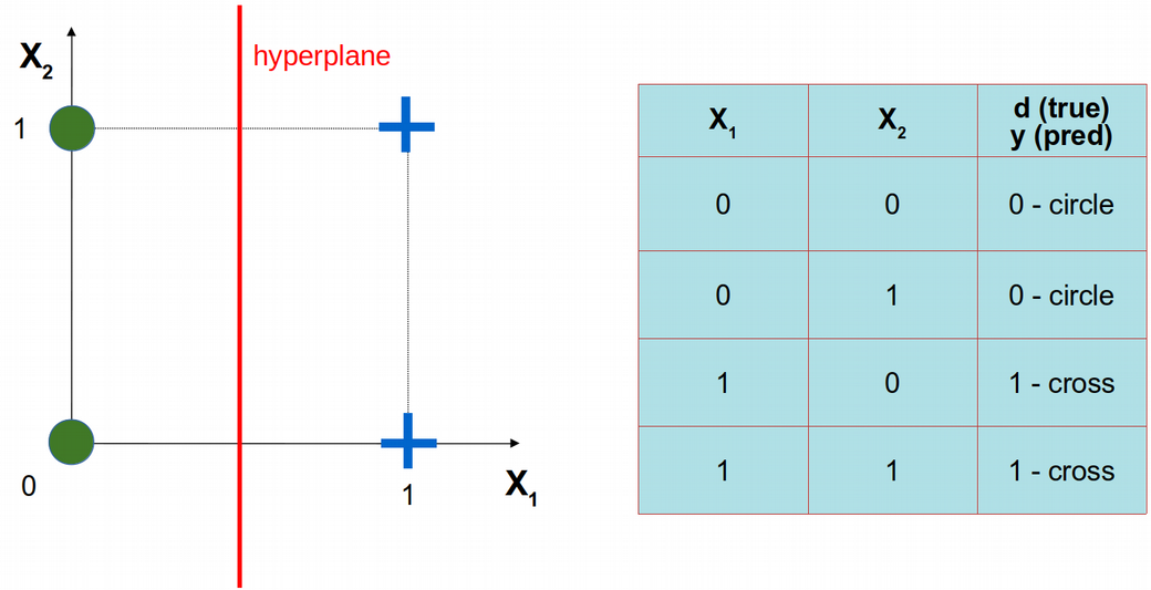
Let us consider a simple problem of only two features, i.e. \(X_1\) and \(X_2\), and only four statistical observations (data points) that belong to two classes: circles and crosses. The four data points are schematically depicted below using \(X_1\) vs. \(X_2\) coordinate system. Obviously, the circles and crosses are separable with a linear decision boundary, i.e. hyperplane.
Let us implement the simplest possible feedforward / dense Artificial Neural Network (ANN) without hidden layers using Keras / Tensorflow library. Later, we will reproduce the results from Keras using from scratch coding ANN in R.
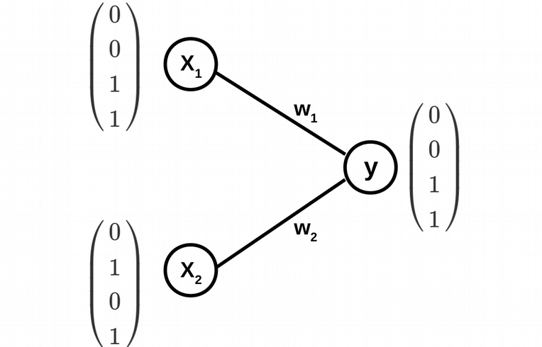
The architecture of the simplest ANN is displayed above, and includes two input nodes (two feature vectors \(X_1\) and \(X_2\)) and one output node, where the two classes are coded in the following way: circles are codded as 0 and crosses as 1. The weights \(w_1\) and \(w_2\) of the edges of the ANN graph are the fitting parameters of the model.
2 Keras solution
Let us first define the X matrix of the feature vectors and the y vector of the class labels:
X <- matrix(c(c(0, 0, 1, 1), c(0, 1, 0, 1)), ncol = 2)
X
[,1] [,2]
[1,] 0 0
[2,] 0 1
[3,] 1 0
[4,] 1 1y <- c(0, 0, 1, 1)
y[1] 0 0 1 1Now, let us define a sequential Keras model of the ANN corresponding to the scheme above and print the summary of the model. Here, we are going to use Sigmoid activation function on the output node because we have a binary classification problem.
library(keras)
model <- keras_model_sequential()
model <- model %>%
  layer_dense(units = 1, activation = 'sigmoid', input_shape = c(2))
summary(model)
Model: "sequential"
________________________________________________________________________________
Layer (type) Output Shape Param #
================================================================================
dense (Dense) (None, 1) 3
================================================================================
Total params: 3
Trainable params: 3
Non-trainable params: 0
________________________________________________________________________________Next, we are going to compile and fit the Keras ANN model. Again, for simplicity, we are going to use Mean Squared Error (MSE) loss function, and Stochastic Gradient Descent (SGD) as an optimization algorithm (with a high learning rate 0.1). The training will be for 3000 epochs, it should be enough for MSE to reach zero.
model %>%
  compile(loss = 'mean_squared_error',optimizer = optimizer_sgd(lr = 0.1))
history <- model %>% fit(X, y, epochs = 10000)plot(history$metrics$loss~seq(1:length(history$metrics$loss)),
xlab="Epochs",ylab="Loss",col="blue",cex=0.5)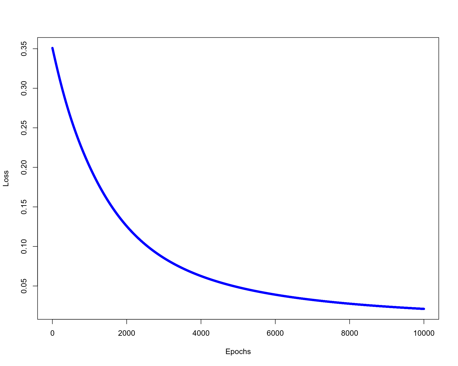
Finally, we will make predictions on the same data set. Overfitting is not a concern here because we want to make sure that the model was capable of linearly separating the two classes of data points.
model %>% predict(X) [,1]
[1,] 0.1748300
[2,] 0.1436723
[3,] 0.8853564
[4,] 0.8594609model %>% predict(X) %>% `>`(0.5) %>% k_cast("int32")tf.Tensor(
[[0]
[0]
[1]
[1]], shape=(4, 1), dtype=int32)It looks like the Keras model successfully can assign correct labels to the four data points.
3 Coding ANN from scratch in R
Now we are going to implement the same ANN architecture from scratch in R. This will allow us to better understand the concepts like learning rate, gradient descent as well as to get an intuition of forward- and back-propagation. First of all, let us denote the sigmoid activation function on the output node as
\[\phi(s)=\frac{1}{1+\exp^{\displaystyle -s}}\]
The beauty of this function is that it has a simple derivative that is expressed through the sigmoid function itself:
\[\phi^\prime(s)=\phi(s)\left(1-\phi(s)\right)\]
Next, the loss MSE function, i.e. the squared difference between the prediction y and the truth d, is given by the following simple equation:
\[E(w_1,w_2)=\frac{1}{2}\sum_{i=1}^N\left(d_i-y_i(w_1,w_2)\right)^2; \,\,\,\,\, y(w_1,w_2)=\phi(w_1x_1+w_2x_2)\]
Finally, the gradient descent update rule can be written as follows:
\[w_{1,2}=w_{1,2}-\mu\frac{\partial E}{\partial w_{1,2}}\]
\[\frac{\partial E}{\partial w_{1,2}}=-(d-y)*y*(1-y)*x_{1,2}\]
where \(\mu\) is a learning rate. Let us put it all together in a simple for-loop that updates the fitting parameters \(w_1\) and \(w_2\) via minimizing the mean squared error:
phi <- function(x){return(1/(1 + exp(-x)))}

X <- matrix(c(c(0, 0, 1, 1), c(0, 1, 0, 1)), ncol = 2)
d <- matrix(c(0, 0, 1, 1), ncol = 1)

mu <- 0.1; N_epochs <- 10000; E <- vector()
w <- matrix(c(0.1, 0.5), ncol = 1) #initialization of weights w1 and w2
for(epochs in 1:N_epochs)
{
  #Forward propagation
  y <- phi(X %*% w - 3) #here for simplicity we use fixed bias = -3

  #Backward propagation
  E <- append(E, sum((d-y)^2))
  dE_dw <- (d-y) * y * (1-y)
  w <- w + mu * (t(X) %*% dE_dw)
}
plot(E ~ seq(1:N_epochs), cex = 0.5, xlab = "Epochs", ylab = "Error", col="red")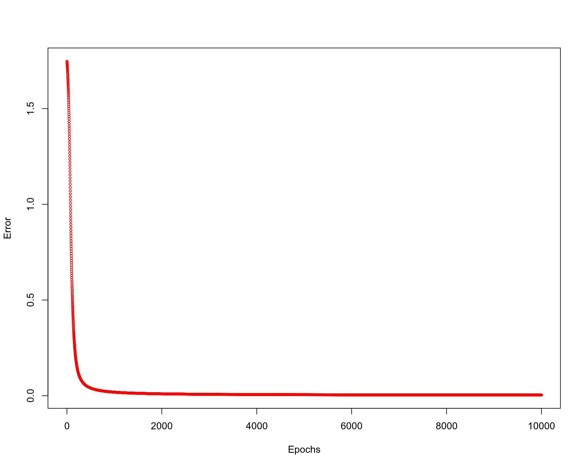
The mean squared error seems to be decreasing and reaching zero. Let us display the final y vector of predicted labels, it should be equal to the d vector of true labels.
y [,1]
[1,] 0.04742587
[2,] 0.03166204
[3,] 0.98444378
[4,] 0.97650411Indeed, the predicted values of labels are very close to the true ones and similar to the ones obtained from Keras solution. Well done, we have successfully implemented an ANN from scratch in R!