Overview
Teaching: 0 min
Exercises: 0 minQuestions
All exercises in this lesson are listed below. The exercises is also included in the different episodes.
1. First steps in R
Challenge 1.1
What are the values after each statement in the following?
mass <- 47.5            # mass?
age  <- 122             # age?
mass <- mass * 2.0      # mass?
age  <- age - 20        # age?
mass_index <- mass/age  # mass_index?
Challenge 1.2
- We’ve seen that atomic vectors can be of type character, numeric (or double), integer, and logical. But what happens if we try to mix these types in a single vector?
Answer
R implicitly converts them all to be the same type.
What will happen in each of these examples? (hint: use
class()to check the data type of your objects):num_char <- c(1, 2, 3, "a") num_logical <- c(1, 2, 3, TRUE) char_logical <- c("a", "b", "c", TRUE) tricky <- c(1, 2, 3, "4")Why do you think it happens?
Answer
Vectors can be of only one data type. R tries to convert (coerce) the content of this vector to find a “common denominator” that doesn’t lose any information.
How many values in
combined_logicalare"TRUE"(as a character) in the following example (reusing the 2..._logicals from above):combined_logical <- c(num_logical, char_logical)Answer
Only one. There is no memory of past data types, and the coercion happens the first time the vector is evaluated. Therefore, the
TRUEinnum_logicalgets converted into a1before it gets converted into"1"incombined_logical.
- You’ve probably noticed that objects of different types get converted into a single, shared type within a vector. In R, we call converting objects from one class into another class coercion. These conversions happen according to a hierarchy, whereby some types get preferentially coerced into other types. Can you draw a diagram that represents the hierarchy of how these data types are coerced?
Answer
logical → numeric → character ← logical
Challenge 1.3 (optional)
- Can you figure out why
"four" > "five"returnsTRUE?Answer
When using “>” or “<” on strings, R compares their alphabetical order. Here “four” comes after “five”, and therefore is “greater than” it.
Challenge 1.4
Using this vector of heights in inches, create a new vector,
heights_no_na, with the NAs removed.heights <- c(63, 69, 60, 65, NA, 68, 61, 70, 61, 59, 64, 69, 63, 63, NA, 72, 65, 64, 70, 63, 65)Use the function
median()to calculate the median of theheightsvector.Use R to figure out how many people in the set are taller than 67 inches.
Solution
heights <- c(63, 69, 60, 65, NA, 68, 61, 70, 61, 59, 64, 69, 63, 63, NA, 72, 65, 64, 70, 63, 65)

# 1.
heights_no_na <- heights[!is.na(heights)]
# or
heights_no_na <- na.omit(heights)
# or
heights_no_na <- heights[complete.cases(heights)]

# 2.
median(heights, na.rm = TRUE)
[1] 64# 3. heights_above_67 <- heights_no_na[heights_no_na > 67] length(heights_above_67)[1] 6
2. Starting with data
Loading the Hawks dataset
| Column | Description |
|---|---|
| Month | 8=September to 12=December |
| Day | Date in the month |
| Year | Year: 1992-2003 |
| CaptureTime | Time of capture (HH:MM) |
| ReleaseTime | Time of release (HH:MM) |
| BandNumber | ID band code |
| Species | CH=Cooper’s, RT=Red-tailed, SS=Sharp-shinned |
| Age | A=Adult or I=Immature |
| Sex | F=Female or M=Male |
| Wing | Length (in mm) of primary wing feather from tip to wrist it attaches to |
| Weight | Body weight (in gram) |
| Culmen | Length (in mm) of the upper bill from the tip to where it bumps into the fleshy part of the bird |
| Hallux | Length (in mm) of the killing talon |
| Tail | Measurement (in mm) related to the length of the tail (invented at the MacBride Raptor Center) |
| StandardTail | Standard measurement of tail length (in mm) |
| Tarsus | Length of the basic foot bone (in mm) |
| WingPitFat | Amount of fat in the wing pit |
| KeelFat | Amount of fat on the breastbone (measured by feel) |
| Crop | Amount of material in the crop, coded from 1=full to 0=empty |
The “Hawks” dataset is available from the RDatasets website.
download.file(
  url = "https://nbisweden.github.io/module-r-intro-dm-practices/data/Hawks.csv",
  destfile = "data_raw/Hawks.csv"
)
## load the tidyverse packages, incl. dplyr
library(tidyverse)
hawks <- read_csv("data_raw/Hawks.csv")
Inspecting data frames
- Size:
dim(hawks)- returns a vector with the number of rows in the first element, and the number of columns as the second element (the dimensions of the object)nrow(hawks)- returns the number of rowsncol(hawks)- returns the number of columns
- Content:
head(hawks)- shows the first 6 rowstail(hawks)- shows the last 6 rows
- Names:
names(hawks)- returns the column names (synonym ofcolnames()fordata.frameobjects)rownames(hawks)- returns the row names
- Summary:
str(hawks)- structure of the object and information about the class, length and content of each columnsummary(hawks)- summary statistics for each column
Note: most of these functions are “generic”, they can be used on other types of
objects besides data.frame.
Challenges
Challenge 2.1
Based on the output of
str(hawks), can you answer the following questions?
- What is the class of the object
hawks?- How many rows and how many columns are in this object?
Solution
str(hawks)spec_tbl_df [908 × 19] (S3: spec_tbl_df/tbl_df/tbl/data.frame) $ Month : num [1:908] 9 9 9 9 9 9 9 9 9 9 ... $ Day : num [1:908] 19 22 23 23 27 28 28 29 29 30 ... $ Year : num [1:908] 1992 1992 1992 1992 1992 ... $ CaptureTime : chr [1:908] "13:30" "10:30" "12:45" "10:50" ... $ ReleaseTime : 'hms' num [1:908] NA NA NA NA ... ..- attr(*, "units")= chr "secs" $ BandNumber : chr [1:908] "877-76317" "877-76318" "877-76319" "745-49508" ... $ Species : chr [1:908] "RT" "RT" "RT" "CH" ... $ Age : chr [1:908] "I" "I" "I" "I" ... $ Sex : chr [1:908] NA NA NA "F" ... $ Wing : num [1:908] 385 376 381 265 205 412 370 375 412 405 ... $ Weight : num [1:908] 920 930 990 470 170 1090 960 855 1210 1120 ... $ Culmen : num [1:908] 25.7 NA 26.7 18.7 12.5 28.5 25.3 27.2 29.3 26 ... $ Hallux : num [1:908] 30.1 NA 31.3 23.5 14.3 32.2 30.1 30 31.3 30.2 ... $ Tail : num [1:908] 219 221 235 220 157 230 212 243 210 238 ... $ StandardTail: num [1:908] NA NA NA NA NA NA NA NA NA NA ... $ Tarsus : num [1:908] NA NA NA NA NA NA NA NA NA NA ... $ WingPitFat : num [1:908] NA NA NA NA NA NA NA NA NA NA ... $ KeelFat : num [1:908] NA NA NA NA NA NA NA NA NA NA ... $ Crop : num [1:908] NA NA NA NA NA NA NA NA NA NA ... - attr(*, "spec")= .. cols( .. Month = col_double(), .. Day = col_double(), .. Year = col_double(), .. CaptureTime = col_character(), .. ReleaseTime = col_time(format = ""), .. BandNumber = col_character(), .. Species = col_character(), .. Age = col_character(), .. Sex = col_character(), .. Wing = col_double(), .. Weight = col_double(), .. Culmen = col_double(), .. Hallux = col_double(), .. Tail = col_double(), .. StandardTail = col_double(), .. Tarsus = col_double(), .. WingPitFat = col_double(), .. KeelFat = col_double(), .. Crop = col_double() .. ) - attr(*, "problems")=<externalptr>
- The object
hawksis of classdata.frame, or more specifically atibble(spec_tbl_df/tbl_df/tbl/data.frame)- Rows and columns: 908 rows and 19 columns
Challenge 2.2
Create a
data.frame(hawks_20) containing only the data in row 20 of thehawksdataset.Notice how
nrow()gave you the number of rows in adata.frame?
- Use that number to pull out just that last row in the data frame.
- Compare that with what you see as the last row using
tail()to make sure it’s meeting expectations.- Pull out that last row using
nrow()instead of the row number.- Create a new data frame (
hawks_last) from that last row.Combine
nrow()with the-notation above to reproduce the behavior ofhead(hawks), keeping just the first 6 rows of the hawks dataset.Solution
## 1.
hawks_20 <- hawks[20, ]
## 2.
# Saving `n_rows` to improve readability and reduce duplication
n_rows <- nrow(hawks)
hawks_last <- hawks[n_rows, ]
## 3.
hawks_head<- hawks[-(7:n_rows), ]
Challenge 2.3
Change the columns
SpeciesandAgein thehawksdata frame into factors.Using the functions you have learnt so far, can you find out…
- How many levels are there in the
Agecolumn?- How many observed birds are listed as females?
Solution
hawks$Species <- factor(hawks$Species)
hawks$Age <- factor(hawks$Age)
nlevels(hawks$Age)
[1] 2summary(hawks$Sex)Length Class Mode 908 character character
- How many levels in the
Agecolumn? There are 2 levels.- How many are listed as females? There are 174 listed as females.
Challenge 2.4
- Store a copy of the factor column
Ageto a new object namedage.- In the new object, rename “A” and “I” to “Adult” and “Immature”, respectively.
- Reorder the factor levels so that “Immature” comes before “Adult”.
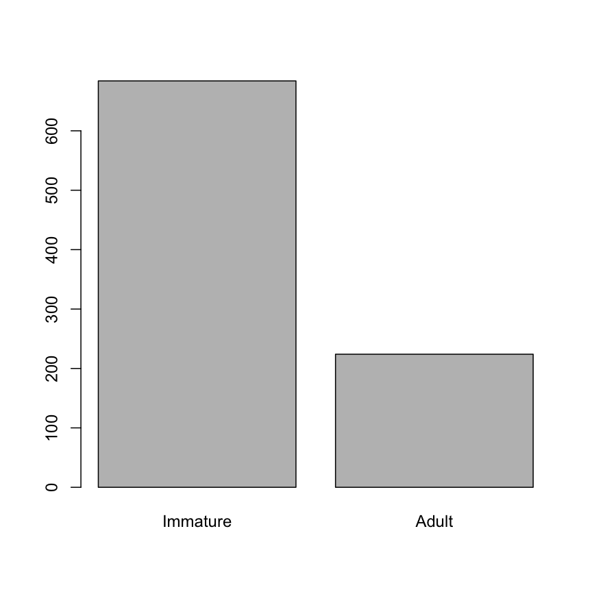
- Create a bar plot of the factor.
Solution
age <- factor(hawks$Age)
levels(age)[1:2] <- c("Adult", "Immature")
age <- factor(age, levels = c("Immature", "Adult"))
plot(age)
Challenge 2.5 (optional)
We have seen how data frames are created when using
read_csv(), but they can also be created by hand with thedata.frame()function. There are a few mistakes in this hand-crafteddata.frame. Can you spot and fix them? Don’t hesitate to experiment!animal_data <- data.frame( animal = c(dog, cat, sea cucumber, sea urchin), feel = c("furry", "squishy", "spiny"), weight = c(45, 8 1.1, 0.8) )Can you predict the class for each of the columns in the following example? Check your guesses using
str(country_climate):
- Are they what you expected? Why? Why not?
- What would you need to change to ensure that each column had the accurate data type?
 country_climate <- data.frame(
        country = c("Canada", "Panama", "South Africa", "Australia"),
        climate = c("cold", "hot", "temperate", "hot/temperate"),
        temperature = c(10, 30, 18, "15"),
        northern_hemisphere = c(TRUE, TRUE, FALSE, "FALSE"),
        has_kangaroo = c(FALSE, FALSE, FALSE, 1)
        )
Solution
- missing quotations around the names of the animals
- missing one entry in the
feelcolumn (probably for one of the furry animals)- missing one comma in the
weightcolumncountry,climate,temperature, andnorthern_hemisphereare characters;has_kangaroois numeric- using
factor()one could replace character columns with factors columns- removing the quotes in
temperatureandnorthern_hemisphereand replacing 1 by TRUE in thehas_kangaroocolumn would give what was probably intended
3. Manipulating, analyzing and exporting data with tidyverse
Useful dplyr functions
select(): subset columnsfilter(): subset rows on conditionsmutate(): create new columns by using information from other columnsgroup_by()andsummarize(): create summary statistics on grouped dataarrange(): sort resultscount(): count discrete values
Challenges
Challenge 3.1
Using pipes, subset the
hawksdata to include only males with a weight (columnWeight) greater than 500 g, and retain only the columnsSpeciesandWeight.Solution
hawks %>%
 filter(Sex == "M" & Weight > 500) %>%
 select(Species, Weight)
# A tibble: 5 × 2 Species Weight <fct> <dbl> 1 CH 550 2 SS 550 3 CH 742 4 SS 1094 5 RT 1080
Challenge 3.2
Create a new data frame from the
hawksdata that meets the following criteria: contains only theSpeciescolumn and a new column calledTarsus_cmcontaining theTarsusvalues (currently in mm) converted to centimeters. Furthermore, include only values in theTarsus_cmcolumn that are less than 6 cm.Hint: think about how the commands should be ordered to produce this data frame!
Solution
hawks_tarsus_cm <- hawks %>%
    mutate(Tarsus_cm = Tarsus / 10) %>%
    filter(Tarsus_cm < 6) %>%
    select(Species, Tarsus_cm)
Challenge 3.3
Use the function
kg_to_lb()above to create a new column in thehawksdata frame with the body weight expressed in pounds.Solution
hawks %>%
    mutate(Weight_lb = kg_to_lb(Weight / 1000))
Challenge 3.4
- For each year in the
hawksdata frame, how many captured birds have a weigh greater than 500 g?Solution
hawks %>%
 filter(Weight > 500) %>%
 count(Year)
# A tibble: 12 × 2 Year n <dbl> <int> 1 1992 33 2 1993 28 3 1994 90 4 1995 56 5 1996 14 6 1997 45 7 1998 26 8 1999 57 9 2000 82 10 2001 37 11 2002 61 12 2003 58
Use
group_by()andsummarize()to find the mean and standard deviation of the weight for each species and sex.Hint: calculate the standard deviation with the
sd()function.Solution
hawks %>%
    group_by(Species, Sex) %>%
    summarize(mean = mean(Weight),
              stdev = sd(Weight))
# A tibble: 9 × 4 # Groups: Species [3] Species Sex mean stdev <fct> <chr> <dbl> <dbl> 1 CH F 490. 183. 2 CH M 348. 99.1 3 CH <NA> 402 110. 4 RT F 1147. 46.2 5 RT M 1080 NA 6 RT <NA> NA NA 7 SS F NA NA 8 SS M NA NA 9 SS <NA> 95 NA
4. Data Visualization with ggplot2
The grammar
ggplot(data = <DATA>, mapping = aes(<MAPPINGS>)) + <GEOM_FUNCTION>() + ...
Challenges
Challenge 4.1
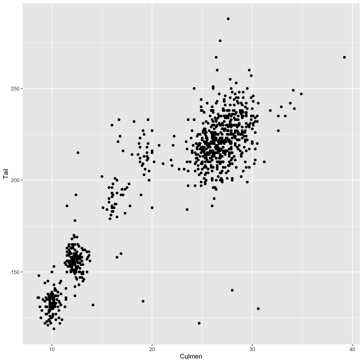
Create a scatter plot with the culmen length (column
Culmen) plotted against the tail length (columnTail).Solution
ggplot(data = hawks,
       mapping = aes(x = Culmen, y = Tail)) +
  geom_point()
Warning: Removed 7 rows containing missing values (geom_point).
Challenge 4.2
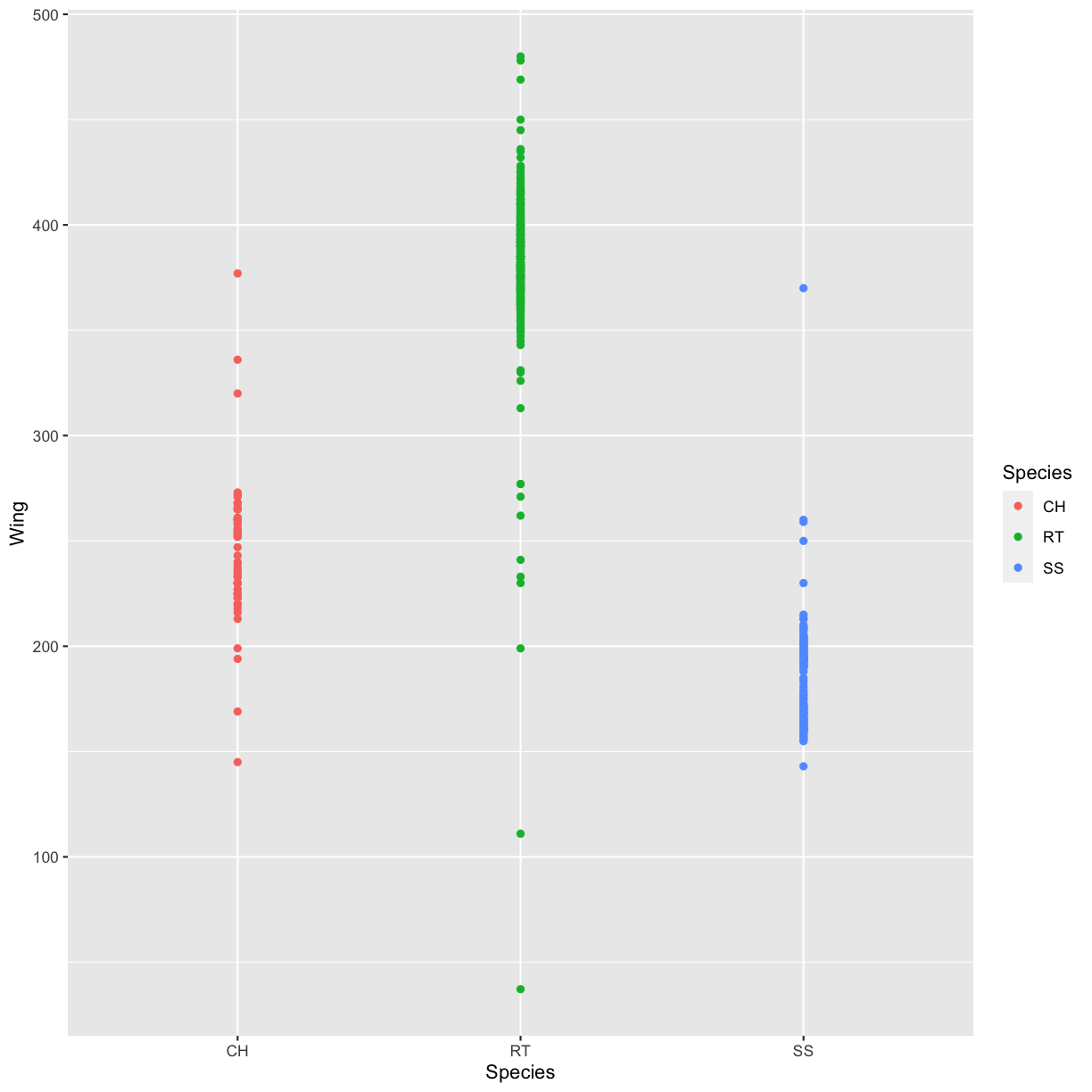
Use what you just learned to create a scatter plot of the species (column
Species) against the wing length (columnWing). Is this a good way to show this type of data?Solution
ggplot(data = hawks,
       mapping = aes(x = Species, y = Wing)) +
  geom_point(aes(color = Species))
Warning: Removed 1 rows containing missing values (geom_point).
Challenges 4.3
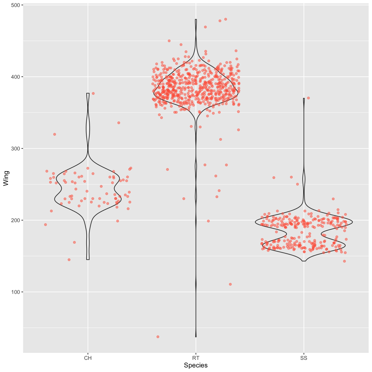
Boxplots are useful summaries, but hide the shape of the distribution. For example, if there is a bimodal distribution, it would not be observed with a boxplot. An alternative to the boxplot is the violin plot (sometimes known as a beanplot), where the shape (of the density of points) is drawn. Replace the box plot with a violin plot; see
geom_violin(). Modify the code below to show a violin plot instead.ggplot(data = hawks, mapping = aes(x = Species, y = Wing)) + geom_boxplot(alpha = 0) + geom_jitter(alpha = 0.5, color = "tomato")Solution
ggplot(data = hawks, mapping = aes(x = Species, y = Wing)) +
    geom_violin(alpha = 0) +
    geom_jitter(alpha = 0.5, color = "tomato")
Warning: Removed 1 rows containing non-finite values (stat_ydensity).Warning: Removed 1 rows containing missing values (geom_point).
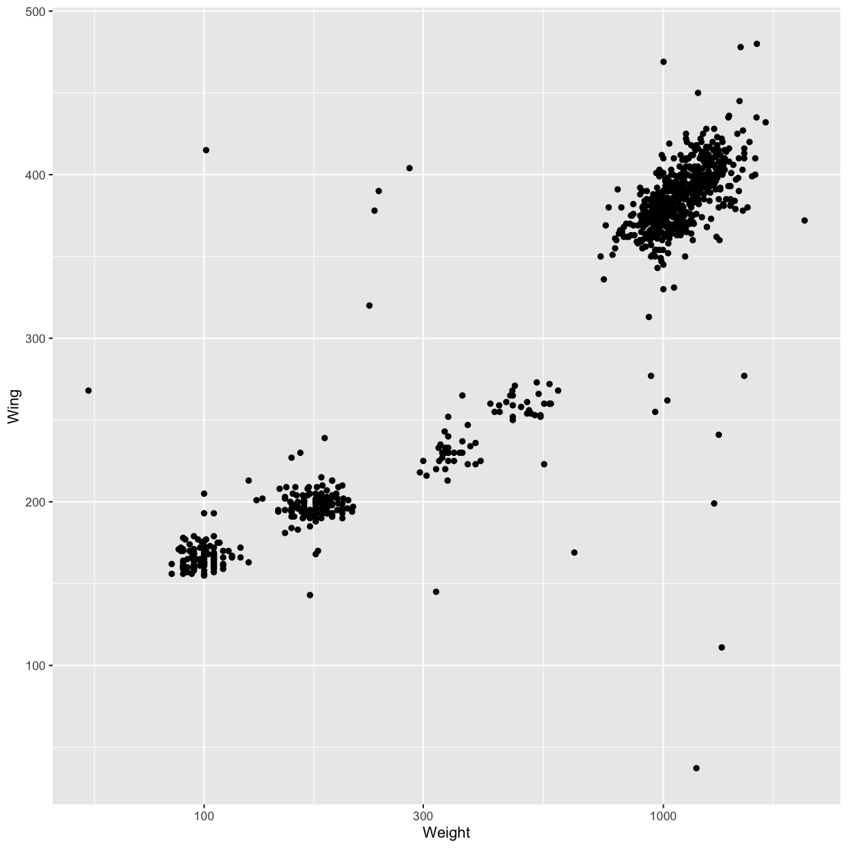
In many types of data, it is important to consider the scale of the observations. For example, it may be worth changing the scale of the axis to better distribute the observations in the space of the plot. Changing the scale of the axes is done similarly to adding/modifying other components.
- Modify the code below so that weight is shown on a log 10 scale; see
scale_x_log10().ggplot(data = hawks, mapping = aes(x = Weight, y = Wing)) + geom_point(alpha = 0)Solution
ggplot(data = hawks, mapping = aes(x = Weight, y = Wing)) +
  geom_point() +
  scale_x_log10()
Warning: Removed 11 rows containing missing values (geom_point).
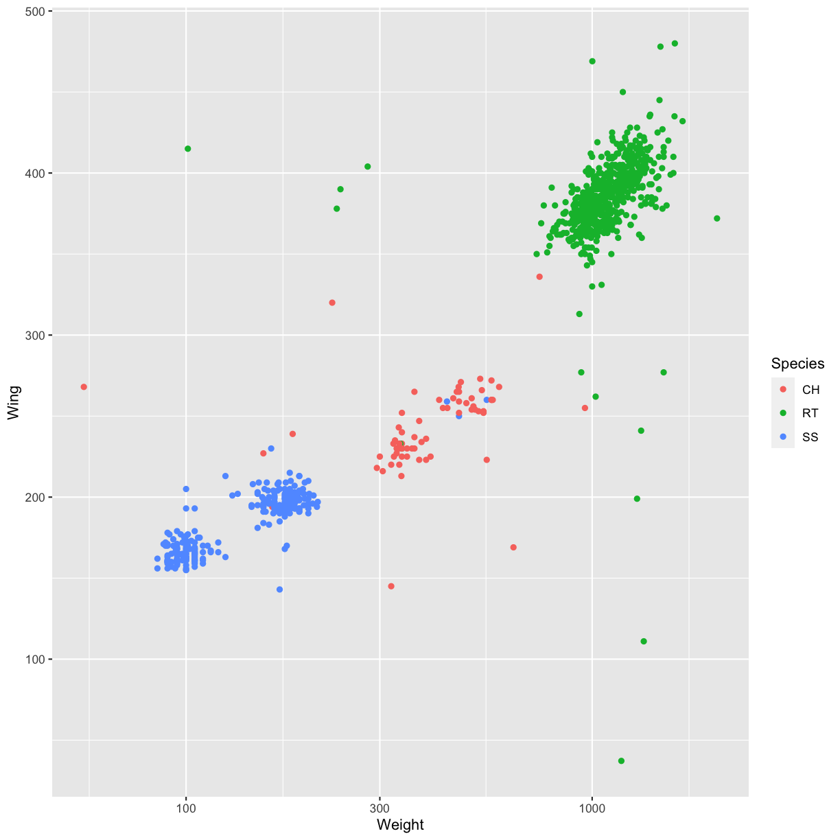
- Add color to the data points on your plot according to the Species.
Solution
ggplot(data = hawks, mapping = aes(x = Weight, y = Wing)) +
  geom_point(aes(color = Species)) +
  scale_x_log10()
Warning: Removed 11 rows containing missing values (geom_point).
Challenge 4.4
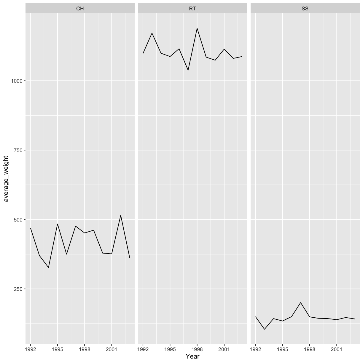
Use what you just learned to create a plot that depicts how the average weight of each species changes through the years.
Solution
yearly_weight <- hawks %>%
  group_by(Species, Year) %>%
  summarize(average_weight = mean(Weight, na.rm = TRUE))

ggplot(data = yearly_weight, aes(x=Year, y = average_weight)) +
  geom_line() + facet_wrap(vars(Species))
Challenge 4.5
With all of this information in hand, please take another five minutes to either improve one of the plots generated in this exercise or create a beautiful graph of your own. Use the RStudio
ggplot2cheat sheet for inspiration.Here are some ideas:
- See if you can change the thickness of the lines.
- Can you find a way to change the name of the legend?
- Try using a different color palette (see http://www.cookbook-r.com/Graphs/Colors_(ggplot2)/).
