NMF - Non-Negative Matrix Factorization

by Sergiu Netotea, NBIS, Chalmers

• Basic NMF presentation and solving
• Comparisons to SvD and PCA. When to use what?
• Toy dataset example
• More complex NMF methods and their applications in omics integration
• NMF for dimensionality reduction (lab)
  • Recommend a multi-omic cause (gene/protein/metabolite) for a phenotipic effect, or the opposite.

Further read:

• Seminal paper: NMF outperforms similar techniques at learning parts representation
• Lee, D., Seung, H. Learning the parts of objects by non-negative matrix factorization. Nature 401, 788–791 (1999). https://doi.org/10.1038/44565

Observations:

• NMF was historically the best hidden feature based image segmentation prior to CNNs
• In comparison to other MF methods (especially the orthogonality enforcing methods), NMF hidden features are not independent, but overlapping, in a hierarchical manner (thus good for hierarchical clustering)

NMF - Non-Negative Matrix Factorization

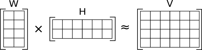
• Matrix factorization (MF): [Credit: Wikipedia]

• Latent (hidden) factors:

  • Each sample can be described by k attributes. Example: How likely is it that a person suffers from a certain type of cancer?
  • Each observation (example: gene) can be described by an analagous set of k attributes or features. Example: How likely is it for the gene to be involved/co-regulated/induced etc in a certain type of cancer. We call such attributes hidden features, or latent factors.
  • Hidden features: We don't always know what these features are, how many are relevant. We learn them, or rather let the machines pick.

• Model constraints: $$ X\in\mathbb{R}_+^{m \times n}, \\ X \approx WH, \\ W \in \mathbb{R}_+^{m \times k}, \\ H \in \mathbb{R}_+^{k \times n} $$

  • NMF is a subtype of matrix factorizations where the additional requirement is that the initial matrix and the decomposed matrices are positive.
  • Why is non-negativity important? It implies the additivity of latent factors.

The Frobenius norm

• Possibly the best way to normalize omics for a joint model. For a m x n matrix A: $$ \| A \|_F = \sqrt{\sum_{i=1}^{m} \sum_{j=1}^{n} |a_{ij}|^2} = \sqrt{\text{trace}(A^T A)} $$
• The Frobenius norm is a way to measure the size or "magnitude" of a matrix, analogous to how the Euclidean norm measures the length of a vector. It is a type of matrix norm and is particularly useful in numerical linear algebra because of its simple interpretation and computational ease.

NMF - some intuitive examples from multi-omics:

V matrix (values matrix)	(weights, scores) W matrix	(hidden, loadings) H matrix
expression values (gene x samples)	genes x factors (metagenes)	factors (metagenes) x samples
protein counts (proteins x samples)	proteins x factors (domains)	factors (domains) x samples
multiomics observations (genes, proteins, etc x samples)	(genes, proteins, etc) x factors (multiomic features)	factors (multiomic features) x samples
multiple datasets (genes x samples x batches)	genes x factors (multi_batch domains)	factors (multi_batch domains) x samples

NMF - in general contexts:

V matrix (values matrix)	(weights, scores) W matrix	(hidden, loadings) H matrix
recommender systems (item x user)	items x factors (preferences)	factors (preferences) x users
collaborative filtering (user x user connections)	user x factors (communities)	factors (communities) x users
language processing (word distribution x document)	word x factors (topics)	factors (topics) x documents
facial recognition (faces x labels)	faces x factors (facial features)	factors (facial features) x labels
microscopy pictures (picture x samples)	pictures x factors (image segments)	factors x samples
spectrometry (spectra x sample)	spectra x factors (component molecules)	factors (component molecules) x samples

Solving NMF

• Similar to ICA, PCA, MFA it can be classified as an unsupervised dimensionality reduction / clustering technique.
• As an optimization problem: $ min~\|X-WH\|_F, V \ge 0, W \ge 0, H \ge 0$
  • With the Frobenius norm, the fit function is: $ F = \sum_{u,i} (x_{ui} - w_u h_i^T)^2, x_{ui} \approx w_u h_i^T = \sum_k{w_{uk} h_{ki}}$
  • This is non convex optimization (no global minima)!
  • The number of latent factors is a result of global fitting
• Many algorithms exist, such as iterated coordinate descent (the original solver), hierarchical alternated least squares.
• Main solver works iteratively via alternating non-negative least squares (ANLS)
• Weak convergence: it is reinitialized several times to avoid local minima, and the best result is kept.
• Since NMF has multiple local minima, starting from different initial values for W and H can lead the algorithm to settle in different parts of the solution space. Some initializations might lead to poor local minima with higher approximation errors, while others might lead to better or more meaningful decompositions.
• Optimal number of k components (hidden atributes) needs fitting (RSS scores for example, Silhouettes scores etc)

Alternating non-negative least squares (ANLS)

• Non-negative least squares problems cannot be solved in a simple closed form, such as in the case of a least square problem. (There is no direct matrix multiplication based solution available). $$ \mbox{minimize } \|Vx-b\|^2 \mbox{ such that } x \geq 0; $$
• The basic idea behind ALS is to alternate between solving for W and H iteratively while keeping the other fixed. Each subproblem is essentially a non-negative least squares (NNLS) problem. $$ \begin{align} W := \operatorname{argmin}_{W \geq 0} \|X-WH\|_F^2 \\ H := \operatorname{argmin}_{H \geq 0} \|X-WH\|_F^2 \end{align} $$
• Thus: $$\begin{align} W_{t+1} &= W_t^T \frac{XH_t^T}{XH_tH_t^T} \\ H_{t+1} &= H_t \frac{W_t^TX}{W^T_tW_tX}. \end{align} $$
• These two steps are repeated iteratively, alternating between solving for W and H until convergence is reached or a stopping criterion is met (such as reaching a certain number of iterations or the error between X and WH becomes sufficiently small.

NMF - multi omics usage observations

• The different omics datasets have different scales and normalities, and this will impact your results (but it also depends on assumptions, on the goal of your study).
• The second problem is enforcing the non-negativity constraint, which might imply additional transformations such as re-scaling and translating
• To bring the different datasets Frobenius norms to the same baseline one can do: $$ X = \begin{bmatrix} \frac{x^{1j}}{\sum_jx^{1j}} / \|\frac{x^{1j}}{\sum_jx^{1j}}\|_F \\ \frac{x^{2j}}{\sum_jx^{2j}} / \|\frac{x^{2j}}{\sum_jx^{2j}}\|_F \\ \vdots \\ \frac{x^{Nj}}{\sum_jx^{Nj}} / \|\frac{x^{Nj}}{\sum_jx^{Nj}}\|_F \\ \end{bmatrix}, $$

Comparison to PCA and autoencoders

• Overall:
  • PCA is good at isolating feature that contain sufficient signal, but will transform the dataset in the direction of maximal variability
  • NMF will not have you lose the original features, you can see it as a data compression tool and has superior interpretability
  • Autoencoders are good for high dimensional complex datasets, but it is difficult to interpret your findings beside a simple clustering
• Factors interpretability:
  • PCA: search for optimal rank k approximations, using it as a linear basis fit to re-write the data.
  • NMF: your data is written as a weighted sum of the basis you learn, but multiple basis can be just as good.
  • Autoencoder: fators are difficult to interpret, but can capture nonlinear effects.
• What it tries to explain:
  • PCA: variation in the data (it is an SvD on the covariation matrix, performing sequential normalizations of data along axes of variation)
  • NMF: additive signal, the very purpose of NMF is to isolate distinct and interpretable signals (paterns) within the data
  • Autoencoder: an autoencoder simply tries to reproduce it's original signal.
• Dimensionality curse:
  • PCA: better at smaller datasets, covariation tends to be equal at large dimensions, good at isolating signal from noise from data
  • NMF: even better at small datasets, provided a good signal fit is found, good at isolating paterns
  • Autoencoder: better at complex and large datasets, were interpretability is not an end goal

Further read:

• https://towardsdatascience.com/step-by-step-signal-processing-with-machine-learning-pca-ica-nmf-8de2f375c422
• https://towardsdatascience.com/autoencoders-vs-pca-when-to-use-which-73de063f5d7
• https://iqbalamo93.medium.com/pca-and-nmf-a-quick-walkthrough-f53d30a968fc

Toy dataset

• Lets pretend that we manage to summarise the effective signal from several omics features in a cheap clinical test.
• Each sample is a private individual. Our test is targeted on one of these afflictions: (cancer, melancholy, diabetes). These are hidden factors: We don't always know what these features are, how many are relevant. We learn them, or rather let the machines pick.
• Each individual is summarised by a few omics features. We will use NMF and collaborative filtering to extract knowledge from such a system.

import pandas as pd
import numpy as np

m = np.array([[0,1,0,1,2,2],
             [0,1,1,1,3,4], 
             [2,3,1,1,2,2],
             [1,1,1,0,1,1],
             [0,2,3,4,1,1],
             [0,0,0,0,1,0]])

dataset = pd.DataFrame(m, columns=['John', 'Alice', 'Mary', 'Greg', 'Peter', 'Jennifer'])
dataset.index = ['diabetes_gene1', 'diabetes_gene2', 'cancer_protein1', 'unclear', 'melancholy_gene', 'cofee_dependency_gene']
V = dataset # we call the initial matrix V
print("\n\n V - Initial Data matrix (features x samples):")
print(V)

 V - Initial Data matrix (features x samples):
                       John  Alice  Mary  Greg  Peter  Jennifer
diabetes_gene1            0      1     0     1      2         2
diabetes_gene2            0      1     1     1      3         4
cancer_protein1           2      3     1     1      2         2
unclear                   1      1     1     0      1         1
melancholy_gene           0      2     3     4      1         1
cofee_dependency_gene     0      0     0     0      1         0

Intuitively we can see that the users (samples) are conected to their items (genes) via a hidden scheme, that could simplify this table. The elements of such a hidden scheme we call hidden (latent) factors. Here is a possible example:

# we estimate k = 3 hidden features
latent_factors = ['latent1', 'latent2',  'latent3']

# For k = 3 we solve the NMF problem
from sklearn.decomposition import NMF

model = NMF(n_components=3, init='random', random_state=0) # define the model
#r = nmf.fit(V)
W = model.fit_transform(V)
H = model.components_

W = pd.DataFrame(np.round(nmf.transform(V),2), columns=H.index)
W.index = V.index
print("\n\n W - factors matrix (features, factors):")
print(W)

 W - factors matrix (features, factors):
                       latent1  latent2  latent3
diabetes_gene1            0.17     0.03     0.37
diabetes_gene2            0.30     0.00     0.58
cancer_protein1           0.07     0.47     0.49
unclear                   0.04     0.21     0.16
melancholy_gene           0.00     0.00     2.29
cofee_dependency_gene     0.04     0.00     0.00

H = pd.DataFrame(np.round(H,2), columns=V.columns)
H.index = latent_factors
print("\n\n H - coefficients matrix (factors, samples):")
print(H)

 H - coefficients matrix (factors, samples):
         John  Alice  Mary  Greg  Peter  Jennifer
latent1  0.00   1.03  1.51  2.04   0.50      0.52
latent2  0.00   0.23  0.00  0.05   1.14      1.40
latent3  0.88   0.96  0.26  0.00   0.21      0.06

Can we figure out the hidden factors? We can do this in one of two ways, if we know the real afflictions, or as it is in our toy model, we only know the effect of our omics features. Thus, we have to look into W (weights or factors matrix)

• melancholy_gene has the strongest weight on latent 3. Latent3 also contains strong weights for all other afflictions but it is separating well only the melancholy factor.
• latent1 contains strong weights for diabetes.
• latent2 contains strong weights for the cancer protein

latent_factors = ['Diabetes', 'Cancer', 'Melancholy']
H = pd.DataFrame(np.round(nmf.components_,2), columns=V.columns)
W = pd.DataFrame(np.round(nmf.transform(V),2), columns=latent_factors)
H.index = latent_factors
W.index = V.index
print(H)
print(W)

            John  Alice  Mary  Greg  Peter  Jennifer
Diabetes    0.00   1.95  0.00  0.41   9.68     11.86
Cancer      4.32   4.96  1.22  0.00   2.48      2.10
Melancholy  0.00   0.88  1.30  1.76   0.43      0.44
                       Diabetes  Cancer  Melancholy
diabetes_gene1             0.17    0.03        0.37
diabetes_gene2             0.30    0.00        0.58
cancer_protein1            0.07    0.47        0.49
unclear                    0.04    0.21        0.16
melancholy_gene            0.00    0.00        2.29
cofee_dependency_gene      0.04    0.00        0.00

Example findings:

• What disease is NMF suspeting for Jennifer? Indeed, it is diabetes. We would not know this from a PCA study, because some of the scores can be negative and so are some of the loadings. The cumulative effect is obscured by the linear transformations.
• The "unclear" feature is strongly related to cancer.

Hypothesis hunting: W x H is an approximation of V, so by transforming the dataset based on the NMF model we can learn some new things.

reconstructed = np.dot(W,H)
reconstructed = pd.DataFrame(np.round(reconstructed,2), columns=V.columns)
reconstructed.index = V.index

print(reconstructed)

                       John  Alice  Mary  Greg  Peter  Jennifer
diabetes_gene1         0.13   0.81  0.52  0.72   1.88      2.24
diabetes_gene2         0.00   1.10  0.75  1.14   3.15      3.81
cancer_protein1        2.03   2.90  1.21  0.89   2.05      2.03
unclear                0.91   1.26  0.46  0.30   0.98      0.99
melancholy_gene        0.00   2.02  2.98  4.03   0.98      1.01
cofee_dependency_gene  0.00   0.08  0.00  0.02   0.39      0.47

• This is the matrix that the model learned by performing NMF. Compared to PCA we kept the original dimensionality. WH is the equigalent of a compression-decompression operation.
• Jennifer and Peter are both suspected diabetes based on their H values.
• Peter is showing signal on the coffee dependency gene in the initial dataset. The model infers that maybe the signal for that gene was lost during processing. The model predicts even higher signal on that gene than Peter has. This is based on how similar Jeniffer is to Peter compared to all the other patients.
• This is the essence of collaborative filtering: People that share the same signals in certain kind of diseases will also share the same signals in some other kind of features.

Why is NMF so important?

• Because it provides an intuitive interpretation of the results, due to its enforcement of the positive values rule.
• The higher the factor weight, the more “determined” the column (segment) is
• First components are more "determined" based on the data.
• During the lab, you will learn to reccomend interesting gene therapies to cancer patients, based on their hidden subtypes!

Reference: For the toy example I drew inspiration from the following Medium article:

• https://medium.com/logicai/non-negative-matrix-factorization-for-recommendation-systems-985ca8d5c16c

NMF usage observations and applications

NMF has many solvers, that are ultra efficient:

• multiplicative update algorithms
• Alternating Least Square
• NMF based on projection gradient algorithms
• PNMF probabilistic nonnegative matrix factorization

Multiple normalities

• A basic transformation to allign the norms was described before!
• However if the omics datasets have widely different distribution it can happen that one omics dataset will drive all variational signal in the data.
• In such case a more thorough transformation may be necessary (for example via methods such as iCluster+, MOFA, etc) prior to applying NMF.

Should data be normalized before coercing it into a matrix factorization model?

• Generally yes, and this generally goes before any application of machine learning to real data.
• If the normalization is a big issue for your data (such as huge differences in scale) then you should opt for Tree Boosting methods (random forest, ensemble learning) or SNF, rather than matrix factorization.
• In matrix factorization the variables are not considered independently, instead everyting is dependent (linearly) on everything else.

Missingness and regularization

• Biological data usually contain missing values. How can the matrix factorization handle it?
• Use initialization methods such as nndsvd that are friendlier towards sparse matrices is number one.
• For the optimization norm I would pick KL if you have large matrices with a lot of missingness. Rather than doing distances KL would evaluate changes in how data is distributed.
• Also note that you can add a regularization term to the fitness function. This does not help directly but in sparse datasets it is easy to get trapped in local optima.

https://scikit-learn.org/stable/modules/generated/sklearn.decomposition.NMF.html

Paper study

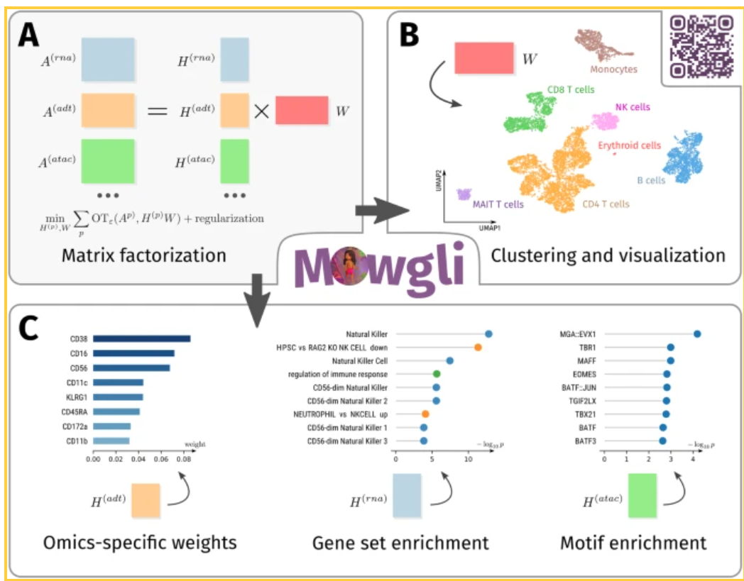
Huizing, GJ., Deutschmann, I.M., Peyré, G. et al. Paired single-cell multi-omics data integration with Mowgli. Nat Commun 14, 7711 (2023). https://doi.org/10.1038/s41467-023-43019-2

• NMF based method for integrating paired single-cell multi-omics data.
• Advancements in single-cell technologies now allow the simultaneous profiling of multiple omics layers (like RNA, chromatin accessibility, and proteins) from the same cells, which raises the need for effective tools to jointly analyze this complex data.
• Combination of Matrix Factorization and Optimal Transport: Mowgli integrates Non-Negative Matrix Factorization (NMF) with Optimal Transport (OT), allowing for both efficient dimensionality reduction and robust alignment of paired omics data. This combination enhances both the clustering accuracy and biological interpretability of the data.
• Integration Across Omics Types: Mowgli is designed to handle various types of omics data, such as scRNA-seq, scATAC-seq, and protein data from modalities like CITE-seq and TEA-seq. This makes it a versatile tool for multi-omics data integration.
• Benchmarking Against State-of-the-Art Methods: Mowgli was benchmarked against other leading methods like Seurat, MOFA+, and Cobolt. It outperformed these methods in embedding and clustering tasks, particularly in scenarios with noisy or sparse data. Mowgli demonstrated superior performance in dealing with real-world challenges like rare cell populations and high dropout rates typical of single-cell data.
• User-Friendly Implementation: Mowgli is implemented as a Python package that integrates seamlessly with popular single-cell analysis frameworks like Scanpy and Muon, making it accessible for researchers.

Paper study:

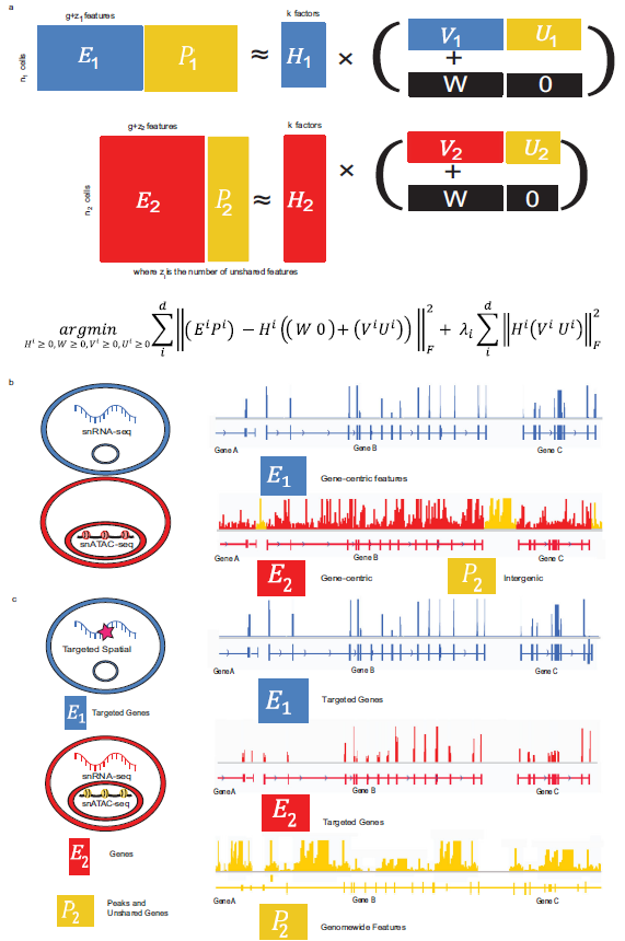
Kriebel, A.R., Welch, J.D. UINMF performs mosaic integration of single-cell multi-omic datasets using nonnegative matrix factorization. Nat Commun 13, 780 (2022). https://doi.org/10.1038/s41467-022-28431-4

• Demonstrates a method for integrating single-cell multi-omic datasets with both shared and unshared features. This is important because many existing integration methods focus only on features shared across datasets (e.g., genes or cells), which limits their ability to fully capture all relevant biological information in complex multi-omic experiments.
• Handling Unshared Features: UINMF is incorporating unshared features — those that appear in only one of the datasets being integrated. This allows it to handle datasets from different omics layers, such as RNA sequencing (scRNA-seq) and chromatin accessibility (snATAC-seq), as well as integrate across different platforms (e.g., spatial and single-cell data).
• The method is applicable in diverse contexts, including:
  • Integrating transcriptomic and epigenomic data.
  • Cross-species data integration, where species-specific genes can be included.
  • Spatial transcriptomic data integration, which typically captures fewer targeted genes compared to full transcriptomes.
• Improved Integration Quality: UINMF was benchmarked against existing methods like iNMF. It consistently showed improved integration quality, especially in scenarios with sparse or heterogeneous data, by leveraging unshared features like intergenic chromatin peaks and species-specific genes.
• Use Cases: The paper demonstrates UINMF’s effectiveness in various scenarios, such as combining scRNA-seq and snATAC-seq data, as well as cross-species integrations where gene sets differ. It shows superior performance in aligning molecular profiles across datasets, which is crucial for understanding complex biological processes.

SNMF - Sparse NMF

• Yuan Gao, George Church, Improving molecular cancer class discovery through sparse non-negative matrix factorization, Bioinformatics, Volume 21, Issue 21, , Pages 3970–3975, https://doi.org/10.1093/bioinformatics/bti653
• Brunet et al., 2004, Metagenes and molecular pattern discovery using matrix factorization PNAS, Mar 2004, 101 (12) 4164-4169; https://doi.org/10.1073/pnas.0308531101

• cancer subtyping in microarrays, dealing with sparse data
• not an integrative example, but one about treating sparsity
• rank estimation of NMF models
• the representation learned is sparse and hierarchical
• $A \approx WH$ The more sparse the matrix of H, the more sparse is the feature matrix W. Therefore, enforcing the sparseness of H will give rise to metagenes that comprised few dominantly deterministic genes.

jNMF - the MOFA of NMFs

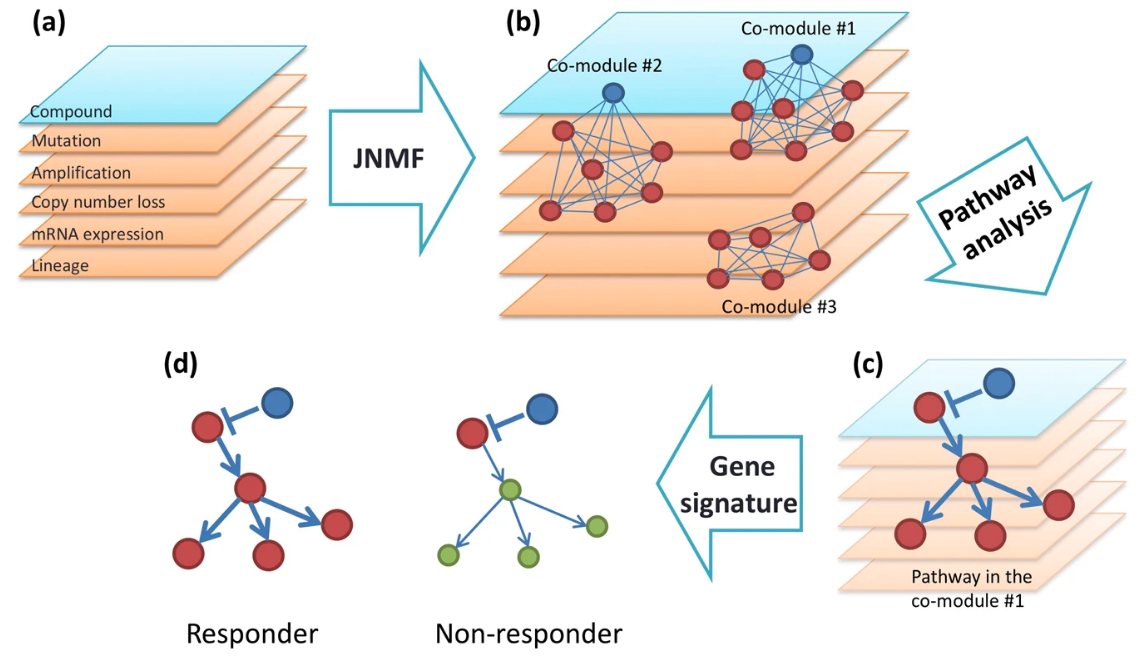
• Fujita, N., Mizuarai, S., Murakami, K. et al. Biomarker discovery by integrated joint non-negative matrix factorization and pathway signature analyses. Sci Rep 8, 9743 (2018). https://doi.org/10.1038/s41598-018-28066-w
• biomarker discovery
• is theoretically and practically equivalent to a standard NMF method with concatenated inputs
• common clusters (co-modules) from mRNA expression, microRNA expression, and DNA methylation data of cancer patients
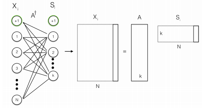
• objective function: $\sum_{i=1}^N \|X_i - WH_i\|$
• NMF method was modified to deal with missingness, by using a mask
• https://rdrr.io/cran/nnTensor/man/jNMF.html
• single cell follow-up: SC-JNMF: Single-cell clustering integrating multiple quantification methods based on joint non-negative matrix factorization, Shiga et al, 2020, preprint at https://www.biorxiv.org/content/10.1101/2020.09.30.319921v1.full.pdf

iNMF - for active learning

• Zi Yang and George Michailidis, A non-negative matrix factorization method for detecting modules in heterogeneous omics multi-modal data, https://doi.org/10.1093/bioinformatics/btv544

• similar to jNMF (based on it) but it uses online learning, this means that one can add information sequentially to improve the model , code here: https://github.com/yangzi4/iNMF

• got a pytorch module: https://pypi.org/project/nmf-torch/

• Used recently in a method for online learning of integrative omics for single cell:

  • Gao, C., Liu, J., Kriebel, A.R. et al. Iterative single-cell multi-omic integration using online learning. Nat Biotechnol (2021). https://doi.org/10.1038/s41587-021-00867-x

Deep NMF - a novel paradigm, doing MF as part of a deep NN

• Flenner, J., & Hunter, B. (2017). A Deep Non-Negative Matrix Factorization Neural Network.
  • https://www1.cmc.edu/pages/faculty/BHunter/papers/deep-negative-matrix.pdf
  • Normal NMF is performed by a single encoding layer

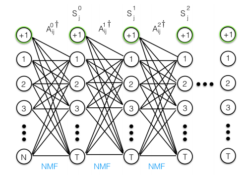
- Deep architecture: CNN, with backpropagation, each NMF layer performs a hierarchical decomposition

• Attention networks
  • NMF can be used to focus attention mechanisms in NNs.
  • Chen et al, Attention-Based Multi-NMF Deep Neural Network with Multimodality Data for Breast Cancer Prognosis Model, Volume 2019 |Article ID 9523719 | https://doi.org/10.1155/2019/9523719

NMF for single cell experiments

• general trends: Bayesian modeling for data sparsity, improvement of model fitting and multi-processing.
• Applications in single cell analysis, pathway enrichment, etc
• Detecting heterogeneity in single-cell RNA-Seq data by non-negative matrix factorization, Zhu et al, 2017, https://pubmed.ncbi.nlm.nih.gov/28133571/

In comparison to other unsupervised clustering methods including K-means and hierarchical clustering, NMF has higher accuracy in separating similar groups in various datasets. We ranked genes by their importance scores (D-scores) in separating these groups, and discovered that NMF uniquely identifies genes expressed at intermediate levels as top-ranked genes.

• CoGAPS 3: Bayesian non-negative matrix factorization for single-cell analysis with asynchronous updates and sparse data structures, Sherman et al, 2020, https://pubmed.ncbi.nlm.nih.gov/33054706/
• Bayesian semi-nonnegative matrix tri-factorization to identify pathways associated with cancer phenotypes, Park et al, https://pubmed.ncbi.nlm.nih.gov/31797616/

Matrix Factorization - beyond NMF

• Scluster method (a mix of MF and SNF): integrates different types of data and maps them into an effective low-dimensional subspace. First, Scluster uses adaptive sparse reduced-rank regression (S-rrr) to map the original data into the principal subspaces. Next, a fused patient-by-patient network is abstracted for these subgroups by a scaled exponential similarity kernel method. It can then obtain the cancer subtypes by spectral clustering.
  • https://pubmed.ncbi.nlm.nih.gov/28113782/
• SRF : rank based multi-view bi-clustering, very related to NMF, possibly reducible to it, it does subtyping and identification of subtype-specific features simultaneously.
  • https://pubmed.ncbi.nlm.nih.gov/27587661/

Software and bibliography:

• Python:
  • recommender systems library: http://surpriselib.com/
  • NMF library: http://nimfa.biolab.si/
  • https://scikit-learn.org/stable/modules/classes.html#module-sklearn.decomposition
• R:
  • general NMF: http://cran.r-project.org/package=NMF
  • usage example: https://compgenomr.github.io/book/biological-interpretation-of-latent-factors.html
  • joint NMF library: https://github.com/rikenbit/nnTensor/
• Deep Semi NMF: https://github.com/trigeorgis/Deep-Semi-NMF

Rank estimation of NMF:

• Jean-Philippe Brunet. et. al., (2004). Metagenes and molecular pattern discovery using matrix factorization. PNAS
• Xiaoxu Han. (2007). CANCER MOLECULAR PATTERN DISCOVERY BY SUBSPACE CONSENSUS KERNEL CLASSIFICATION
• Attila Frigyesi. et. al., (2008). Non-Negative Matrix Factorization for the Analysis of Complex Gene Expression Data: Identification of Clinically Relevant Tumor Subtypes. Cancer Informatics
• Haesun Park. et. al., (2019). Lecture 3: Nonnegative Matrix Factorization: Algorithms and Applications. SIAM Gene Golub Summer School, Aussois France, June 18, 2019
• Chunxuan Shao. et. al., (2017). Robust classification of single-cell transcriptome data by nonnegative matrix factorization. Bioinformatics

Other integrative NMF:

• intNMF: https://journals.plos.org/plosone/article?id=10.1371/journal.pone.0176278
• Simultaneous Non-negative Matrix Factorization (siNMF) : Extracting Gene Expression Profiles Common to Colon and Pancreatic Adenocarcinoma using Simultaneous nonnegative matrix factorization, Liviu Badea, Pacific Symposium on Biocomputing, 13:279-290, 2009,
• Discovery of multi-dimensional modules by integrative analysis of cancer genomic data. Shihua Zhang, et al., Nucleic Acids Research, 40(19), 9379-9391, 2012
• Probabilistic Latent Tensor Factorization, International Conference on Latent Variable Analysis and Signal Separation, Y. Kenan Yilmaz et al., 346-353, 2010

Fast Tensorial Calculus:

• Non-negative Matrix Factorization (NMF) : Nonnegative Matrix and Tensor Factorizations, Andrzej CICHOCK, et. al., 2009,
• A Study on Efficient Algorithms for Nonnegative Matrix/Tensor Factorization, Keigo Kimura, 2017

Non-negative CP Decomposition (NTF)

• α-Divergence (KL, Pearson, Hellinger, Neyman) / β-Divergence (KL, Frobenius, IS) : Non-negative Tensor Factorization using Alpha and Beta Divergence, Andrzej CICHOCKI et. al., 2007, TensorKPD.R (gist of mathieubray)
• Fast HALS : Multi-way Nonnegative Tensor Factorization Using Fast Hierarchical Alternating Least Squares Algorithm (HALS), Anh Huy PHAN et. al., 2008
• α-HALS/β-HALS : Fast Local Algorithms for Large Scale Nonnegative Matrix and Tensor Factorizations, Andrzej CICHOCKI et. al., 2008
• Non-negative Tucker Decomposition (NTD)
  • KL, Frobenius : Nonnegative Tucker Decomposition, Yong-Deok Kim et. al., 2007
  • α-Divergence (KL, Pearson, Hellinger, Neyman) / β-Divergence (KL, Frobenius, IS) : Nonneegative Tucker Decomposition With Alpha-Divergence, Yong-Deok Kim et. al., 2008, Fast and efficient algorithms for nonnegative Tucker decomposition, Anh Huy Phan, 2008
  • Fast HALS : Extended HALS algorithm for nonnegative Tucker decomposition and its applications for multiway analysis and classification, Anh Hyu Phan et. al., 2011